Submarine simulations in one month

Hello again and welcome back! Though it’s only been just over a month since my last post, a lot has changed. Here, I’ll try to explain some of the stuff I’ve learnt, what a general computational fluid dynamics (CFD) simulation is and how one is carried out.

The learning process of completing a CFD simulation is made easier by working with examples further down the simulation line and working your way back up. This is how I’ve learnt to complete the simulations. That being said, I’m worried that writing about the process in that order may make things a tad confusing for the reader (let alone for me writing this). Instead, I’ll explain my experience in the order you’d perform a CFD simulation. Just remember, if you’re considering learning how to do these too, do it in reverse!

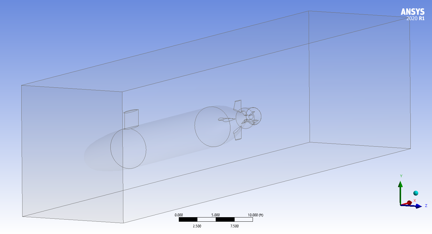
To begin a CFD simulation, you must first define the geometry of your problem – which quite literally means defining the shapes involved. Fortunately, this can be easy when working with simple shapes, like a cube or sphere. Unfortunately for me, submarines can be quite difficult to draw freehand and I was never very good at art. I was thankful to find out that the submarine we are modelling, the DARPA Suboff, has its geometry specifications online which, with a little Python and a lot of luck, can be used to produce the complete geometry in a format we can use.

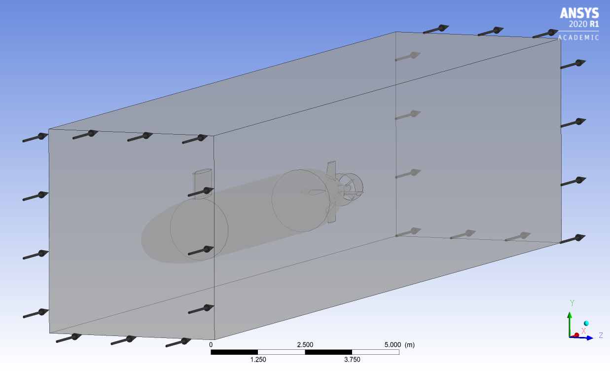
However, to perform any simulations on this, we have to specify boundary conditions (BCs). These BCs include where the fluid is coming from (inlet), where it exits (outlet), and where fluid can go (fluid domain) in the simulation (we’ll come back to these later). With just the submarine in the geometry, we cannot specify where the inlet, outlet, or fluid domain are as the only object that exists is the submarine.

The way CFD fixes this, is by using cavities. This involves creating a large volume in the geometry that encases the submarine (such as a cuboid or cylinder), and then making a submarine-shaped hole inside it. This means we can say the inlet is the front face, the outlet is the back face, and the fluid domain is the volume of the shape that remains after removing the submarine. At this point, it’s important to remember, the fluid cannot enter the cavity. Instead, the fluid domain is just the surrounding volume.

After this, we create a mesh from the geometry. Meshing is a form of approximation that allows for the CFD calculation to take place. This involves splitting the geometry into a set of finite chunks so we don’t have to consider a continuous space. The smaller the chunks, the finer the mesh. So far, the default mesh generated by ANSYS has worked perfectly fine (thankfully), but this may change more precise simulations are required.

The next step is to set up the problem. This involves setting up all the BCs. However, there are many more than the ones I mentioned earlier. These BCs include how the fluid should interact with each face of the geometry, the static pressure of the fluid as it leaves the outlet, and the initial velocity of the fluid. And we still haven’t considered the array of different solvers & methods that can be selected. It goes without saying that that there were a lot of important decisions to be made here, which meant I had a lot more to learn! This involved a bit of reading about CFD and a fair amount of trial and error. As I am writing this, the conditions for my final simulations are still undecided, but I know I’m on the right path.

Once that’s all done, we can begin performing the simulation. Since we have access to an HPC cluster, we can complete such a task much faster with parallelisation – which is quite the upgrade from performing the simulation in serial on your local PC. Those working at the HPC cluster in Luxembourg have done a great job at making the IRIS cluster accessible considering the circumstances. Since most of the heavy lifting has been done in the setup process, at this point the only thing to do is sit back and wait for the cluster to crunch the numbers.

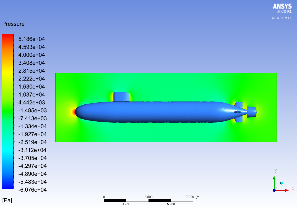
Finally, we arrive at the most exciting part of the process. At this point we see if the conditions we set prior have correctly shown the physical properties we were after – or if we’re heading back to the drawing board. Once the files have transferred from the HPC cluster to your local PC (during which time you could learn an instrument, or count the grains of sand at your local beach) the post-processing begins!

While I initially learnt how to post-process in Paraview, I decided to switch to ANSYS since it’s built into the ANSYS workbench. Within these programs, you are able to select the physical quantities calculated (such as fluid velocity, pressure, temperature etc.) and visualise them on the geometry itself. This allows for a very useful sanity check, as we can see if the simulation has given us physical behaviour, plus we can look at some very cool looking pictures and videos! However, we do still have to work out if what we have simulated is the correct physical behaviour. This means outputting the numerical values of our simulation and comparing these to the values to those calculated in the DARPA Suboff model experiment.

As it stands, I have two weeks remaining to complete the project and can already smell the sweet scent of correct BCs in the air. Hopefully all goes to plan… and I’ll provide an update on the final results in a couple of weeks!

Thanks for reading! Any questions, please let me know in the comments below.