Beware of an accuracy rate that is too high

In machine learning we often talk about accuracy as a metric for how good our model is. Yet a high accuracy isn’t always a good way to measure model performance, nor does it always correlate to an accurate model. In fact, an accuracy rate that is too high, is something to be skeptical about. In machine learning this is something that comes up time after time, you build a model, you get a great accuracy score, you jump with joy, you test it further, you realize that something was wrong all along… you fix it and get a far more reasonable answer…

Side note for the inexperienced reader, if any model or any person tells you that their model predicts the target variable with a 100% accuracy… don’t believe them! How big is their sample size? Are they training and testing their model on the same dataset such that the algorithm simply learns the answer? Have they tested their algorithm on all data we have available for the topic throughout human history? In short, what’s the catch?

In this post I will be talking about how the accuracy metric wasn’t useful in the models I have been building to predict SLURM job run times. In fact, the accuracy metric could even be counterproductive in some scenarios. If you remember from the previous post, estimating predictions of actual job run times could greatly improve the efficiency of Hartree’s cluster scheduling algorithm.

The first model I built was a regression model, given information from the user, like how many CPU’s and nodes they request from the cluster, and what they expect the run time to be, the model tries to predict what the actual run time of each job will be, whilst minimizing the error in prediction. Now in this case, the classic accuracy score isn’t applicable, for regression prediction, things like MSE, mean squared error, are used to estimate the goodness of fit achieved from the model. In the figure below on the left hand side, we can see the red line is the line of best fit for the scattered points. This line minimizes the distance between estimated and actual points. In our case, the line of best fit becomes a bit more complicated. The algorithm my colleague and I are building has the obligation to predict run times such that no run time is underpredicted. That is because in Hartree, similar to many clusters, if the actual run time of a job goes above the provided time limit by the user, the job is killed. So the first and foremost necessity our model has, is that it cannot predict run times lower than the actual time, otherwise the job would then be killed. On the right hand side of the figure we can see how this would look like, the line of best fit is shifted upwards such that no points fall above it.

Now this figure represents a simplistic example, but it is a good way to visualize the problem. In real world problems though the data is much more messy, there are outliers, in both directions that would skew the line of best fit. For our dataset we have an additional complication though, which is presented by the fact that even users sometimes make errors. Users will occasionally submit jobs with runtime predictions that are too low, causing the scheduler to kill their job. These jobs are highly unpredictable and will almost never be accurately estimated by the algorithm. Due to this limitation, we decided construct another model, this time to tackle a classification problem. The idea behind this is that if we were able to classify jobs into two categories, predictable and unpredictable, then we could simply put aside the unpredictable jobs, and run our regression model on the rest, without risking under-predictions and having jobs killed off.

As such we ran our regression model and defined accuracy as whether the run time was predicted correctly above the actual elapsed time (but below the user’s time limit), or incorrectly below it. Having these two classifications we constructed and tested other models like Random Forest Classifier and Naïve Bayes Classifier, to predict the “predictability” of a job. With the accuracy we defined before we had roughly 92% of jobs classified as predictable, and 8% as unpredicatble.

In the first run of a classifier algorithm the code spat out 92% accuracy!!…. Well, that was easy? In fact, too easy. Since algorithms are built to train in such a way that they achieve the highest possible accuracy score, Naïve Bayes simply predicted every job as predictable….oh, so we got 92% accuracy, but in reality that was useless? Yes, the whole point was to distinguish the jobs that are unpredictable, and even with such an “accurate” algorithm, we were nowhere nearer to achieving that task.

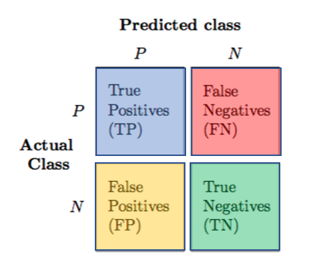
This is one of those scenarios where accuracy scores are misleading. In this case we want to achieve 100% accuracy in predicting “unpredictable” jobs…but remember, what’s the catch? To do this we have to sacrifice accuracy in predicting those jobs which actually are predictable, and misclassify them into the other category. The below image helps to clarify. In our case, think of jobs being predictable as the positive class, while jobs that are not predictable are part of the negative class. Traditional accuracy only looks at the diagonal values of jobs correctly classified as positive or negatives. Other metrics, like recall and precision, take into account the other diagonal of false predictions. In our case we want precision to be 100%, this means that we do not tolerate any false positives (such that negative cases are all correctly labeled). To achieve this though we will generate many false negative cases.

This is it for now folks, we have cornered the best tactic to achieve no under-predictions and now what remains is to optimize the models best we can and test such models on the cluster. We are slightly passed the mid-program mark but I can see the deadlines for the final week approaching. Working on this project has been an amazing experience so far and I have been learning so much thanks to SoHPC, but it’s not time to relax yet .…