And what a dynamic simulation it is!
Finally, we are there: all the data of the runs have been collected and processed, and our hydrogen molecule rotates and vibrates around to make us very happy!
But let’s take a closer look at what we have done, from the beginning:
The aim of our project was to find the ground state of the hydrogen molecule using the VQE’s hybrid Qiskit algorithm, implementing it both locally and in IBM’s real quantum computer. Studying the trend of the curves in the various setting conditions was one of our goals, but the fundamental one was to combine the VQE with the method of quasi-classical trajectories (QCT) in order to obtain and study the dynamics simulations of the molecule. To this end, we solved the system of equations of motion iteratively using the VQE energies calculated at each interatomic distance, using the Runge-Kutta method.
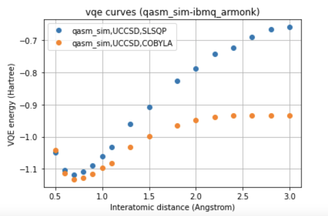
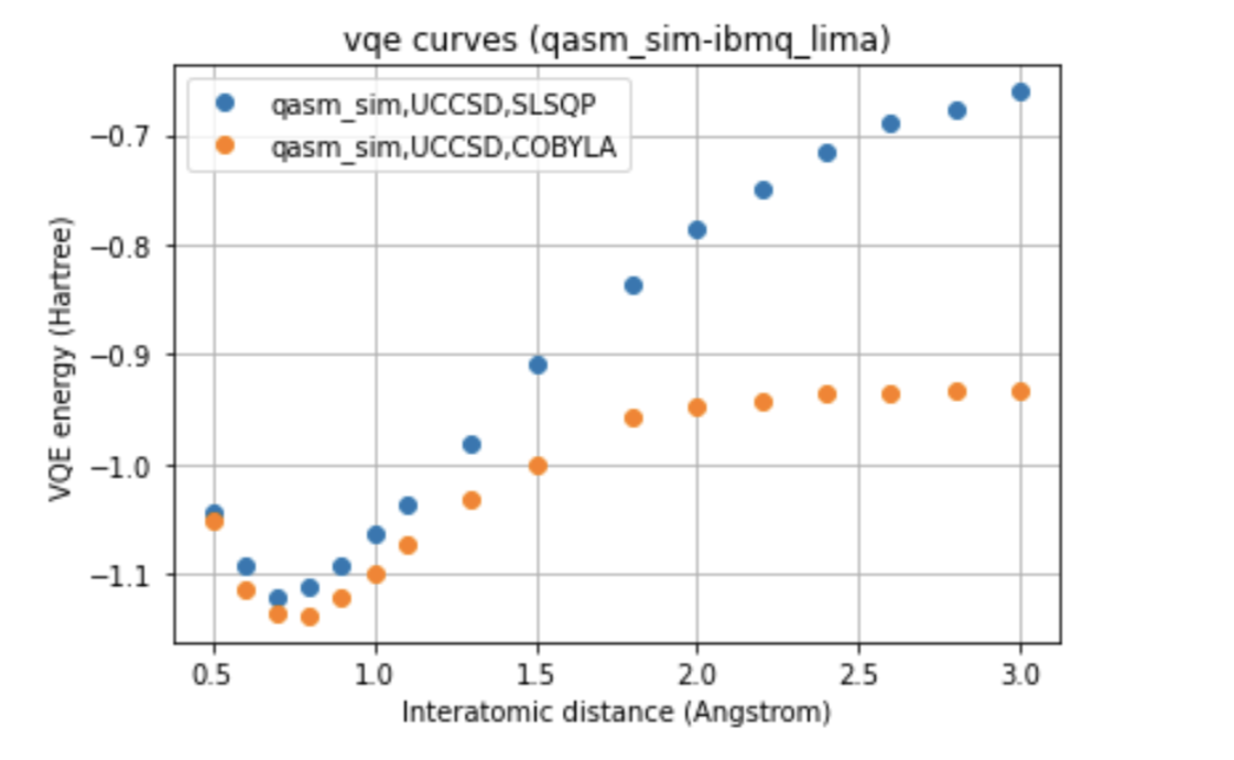
In our work, two different environments were compared for the calculation of the VQE curve, such as statevector simulator, which represents the ideal curve, and qasm simulator, as well as two different optimizers, such as COBYLA and SLSQP, and two different variational forms for the ansatz: UCCSD and SU2.
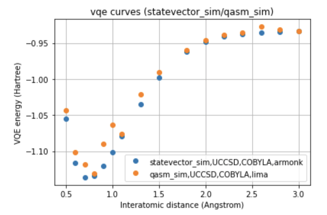
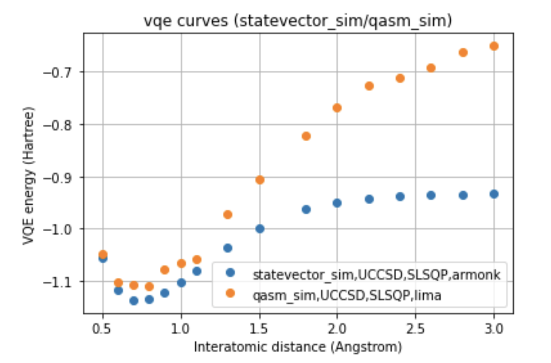
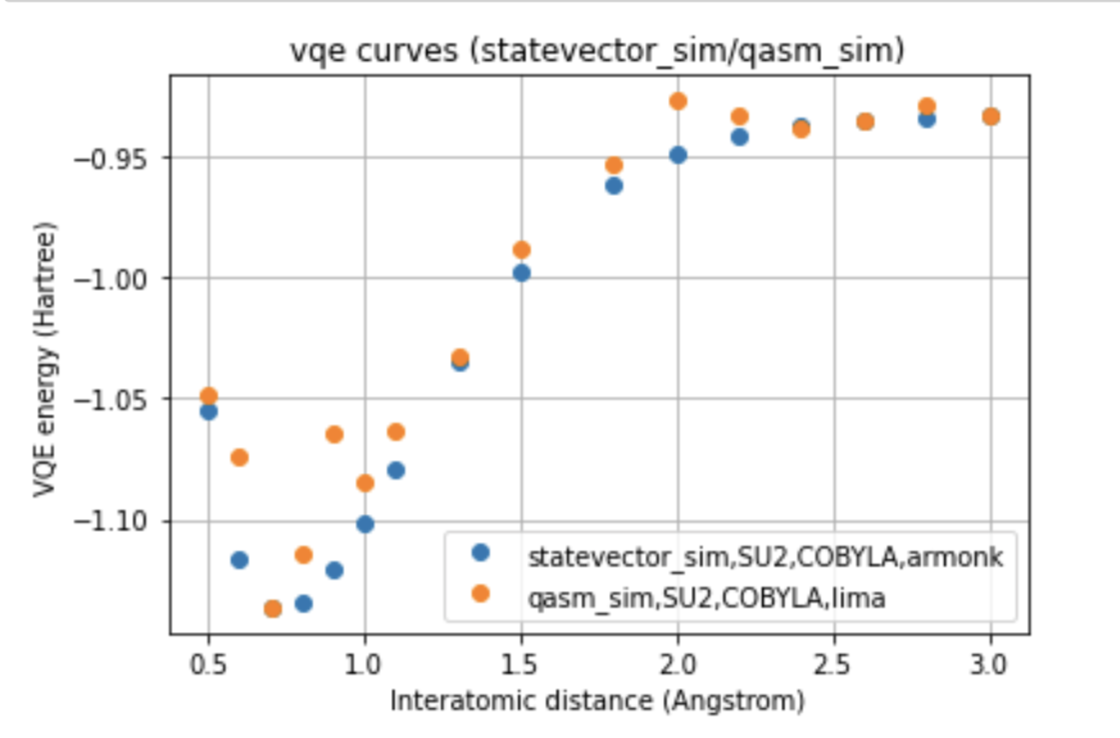
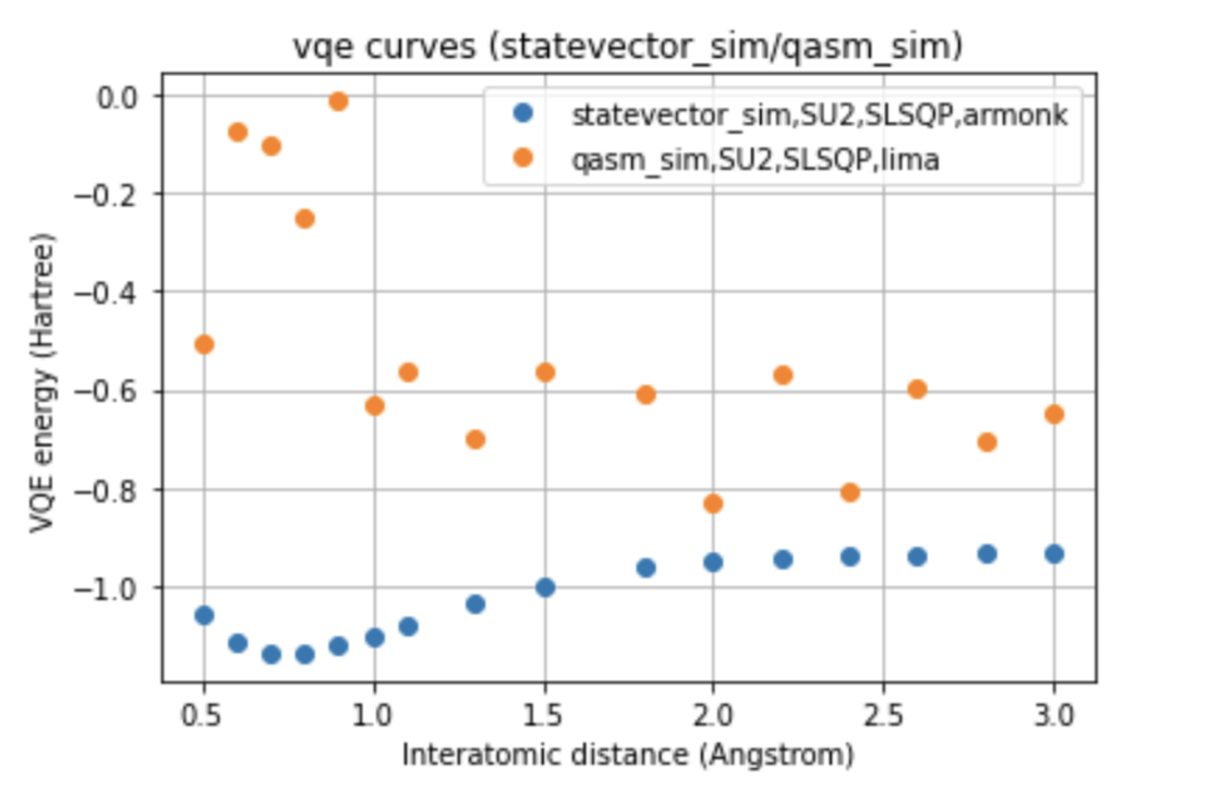
The run was also performed on two different processors, such as Falcon and Canary, to which the ibmq_lima and ibmq_armonk devices correspond. Furthermore, were compared the curves obtained with the noise-model referred to the processors mentioned, and with the noise-mitigations technique, choosing to compare the two different optimizers for each of the variational forms for the run done on the real quantum computer.

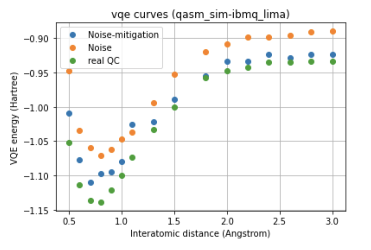
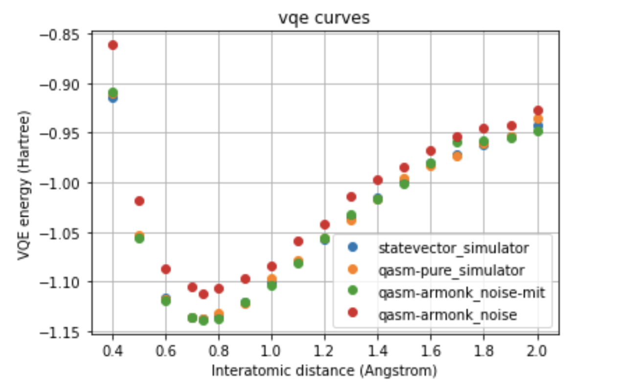
Below we can see a direct comparison between the two different devices respect to the ideal model, images here shown only for a single variational form and for a single optimizer.
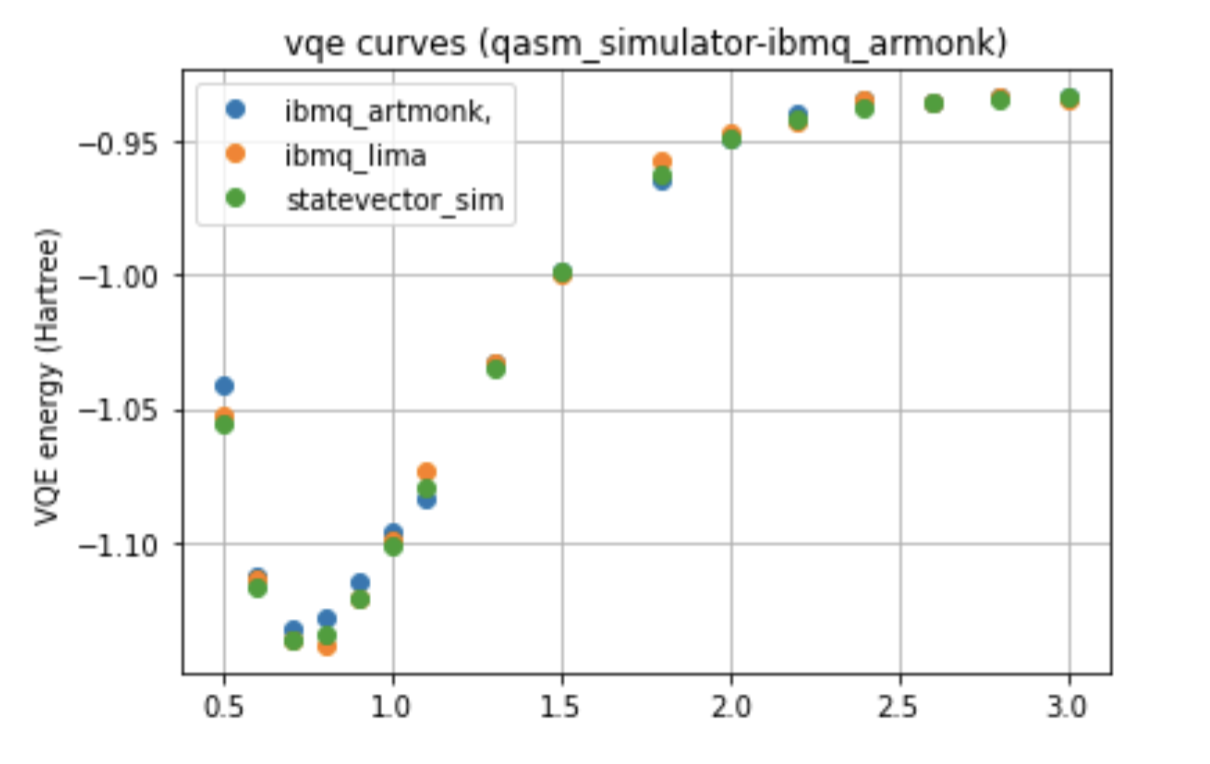
It was chosen also to compare the various techniques with a single device, which is ibmq_armonk, choosing UCCSD as variational form and SPSA as the optimizer.
The most exciting thing was moving on to molecular dynamics simulations. Runs were performed using the environment statevector simulator and with UCCSD as variational form and SPSA as optimizer, which proved useful for converging with less than 200 iterations.
The comparison was made for different initial conditions, where both the vibrations (in which both atoms posses zero momentum) and rotovibrations (which include momentum of both atoms) of the molecule can be observed.

What have we concluded from these results? Well, you just need to read our final report to find out 😉


Leave a Reply