Is benzene a nanotube?

Of course not, but I have input for benzene and I did the first tests of the electron density computation on this system. Before showing the results (Pretty figures!), I would like to tell you about the helical symmetry (something that makes the computation faster) and give some insight into the nanotube code.
Helical symmetry of nanotubes
Tyger Tyger, burning bright,
William Blake: The tyger
In the forests of the night;
What immortal hand or eye,
Could frame thy fearful symmetry?
Symmetry is something that is pleasing for human eye in general, and it has an important role in chemistry as well. The symmetry of molecules is usually described by point groups that contain geometric symmetry operations (mirror plane, rotational axis, inversion center). For example, the water molecule belongs to the C2v point group: it has a mirror plane in the plane of the atoms, another one at the bisector of the bond angle, and a twofold rotational axis, and the identity operator. (I shall note that there is another way to describe the symmetry using permutation of the identical nuclei, which is a more general approach.) Point group symmetry can be used to label the quantum states and it can be incorporated in quantum chemistry programs in a clever way to reduce the cost of the computation.
In my previous post I wrote about how to “make” a nanotube by rolling up a two-dimensional periodic layer of material. The resulting nanotube is periodic along its axis, it has one-dimensional translational symmetry. In the case of a carbon nanotube with R=(4,4) rolling vector the translational unit cell contains 16 carbon atoms (see figure, yellow frame). However, it is better to exploit the helical and translational symmetry (pseudo two-dimensional approach), where the symmetry operation is a rotation followed by a translational step. It this case it is sufficient to use a much smaller unit cell (only two atoms) for the R=(4,4) carbon nanotube. The small unit cell is beneficial because it makes the computation cheaper. The figure below shows the atoms of the central unit cell in red, and the green atoms are generated by applying the rotational-translational operation twice in both directions.

What does the code do?
So, we have a program that can compute the electronic structure of nanotubes (the electronic orbitals and their energies) for a given nuclear configuration. I would like to tell you how it works but I cannot expect you to have years of quantum chemistry study and I don’t want to give you meaningless formulas. Those, who are familiar with the topic can find the details in J. Comput. Chem. 20(2):253-261 and here.
Basis set: Contracted Gaussian basis. The wave function is the linear combination of some basis functions. From the physical point of view the best choice would be using atomic orbitals (s-, p-, d-orbitals), but for a computational reason it is better to use (a linear combination of) Gaussian functions that resemble the atomic orbitals. The more basis functions we use, the better the result will be but the computational cost increases as well.
Level of theory: Hartree-Fock. This is one of the simplest ways to describe the electronic structure. The so-called Fock operator gives us the energy of the electronic orbitals. It is a sum the two terms. The first contains the kinetic energy of the electron, the Coulomb interaction between the electrons and the nuclei, and the internuclear Coulombic repulsion. The second term contains the electron-electron repulsion. The Fock operator is represented by a matrix in the code, and the number of basis functions determines the size of the matrix.
To get the basis function coefficients and the energy we have to compute the eigenvalues of the Fock matrix. To create the matrix we already have to know the electron distribution, so we use an iterative scheme (self consistent field method): Starting from an initial guess, we compute the electronic orbitals, rebuild the Fock matrix with the new orbitals, and diagonalize it again, and so on. The orbital energy computed with an approximate wave function is always greater than the true value, so the energy should decrease during the iteration as the approximation gets better. We continue the iteration until the orbital energies converge to a minimum value. This is how it is done in a general quantum chemistry program, but in our nanotube program it is different, as you will see in the next section.
Transformation to the reciprocal space. The translational periodicity allows us to transform the basis functions from the real space to the reciprocal space (Bloch-orbitals). This way the Fock-matrix will be block diagonal. We diagonalize each block separately, which is a lot cheaper than diagonalizing the whole matrix. This part is parallelized with MPI (Message Passing Interface), each block is diagonalized by a different process.
The results are orbital energies and basis function coefficients for each block. So far the main focus was on the energies (band structure), but now we will something with the orbitals as well.
Finally: the electron density
Now let’s get down to business. The electron density describes the probability of finding the electron at a given point in space, and it is computed as the square of the wave function. Now we are not interested in the total electron density, but the contribution of each electron orbital. For the numerical implementation we have to compute the so-called density matrix from the basis coefficients of the given orbital, and then contract it with the basis functions. First, we compute the electron density corresponding to the central unit cell in a large number of grid points. The electron density of the whole nanotube is computed from the contribution of the central unit cell using the helical symmetry operators.
Electron_density_nanotubeDownload
Let’s see an example, the benzene molecule. (I know it’s not a nanotube, but it’s a small and planar system that is easy to visualize). The unit cell consists of a carbon and a hydrogen atom, and we get the benzene replicating and rotating it six times, and we do the same way for the electron density. This particular orbital shown in the picture is made of the pz-orbital of carbon and the s-orbital of hydrogen. On the left electron density figure, you can see the nodal plane (zero electron density) of pz between the two peaks; and the merging of the pz and the s-orbital to a covalent bond.
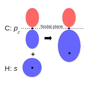
(Grid points are in the plane of the molecule)
The next steps
Recently I have been testing the parallel version of the electron density computation to see if it gives the same result as the serial code or not. I hope it does, so “parallelization” is not among the next steps. (However, one can always improve the code). The next challenge is the visualization of the electron density in 3D.
Hello Everyone, my name is Irén and I am from Budapest. I have just completed my MSc in Chemistry at the Eötvös Loránd University, and now I am applying for the PhD School of Chemistry there. I have always been interested in mathematics and chemistry but I discovered programming only at the university (it was a love at first sight). This is why theoretical computational chemistry became my main topic of interest. This summer I will be staying in Bratislava where I will perform electronic structure computations of nanotubes and optimize the code. I have applied for the Summer of HPC program to study more about parallel programming, to peek into new fields of science and to meet new people.

Leave a Reply