The Clusters of Supercomputers: The Top500 List in the Eyes of Machine Learning

1. Introduction
This summer I started to make my first steps towards the field of HPC. My participation to the SoHPC program sparked my curiosity about this field and I have become willing to learn more about the world’s most powerful supercomputers. The Top500 list has been an interesting source of information to learn about that. I enjoy going through the list and exploring the specifications of those extraordinary computers.
One idea that came across my mind was to apply Machine Learning (ML) to the Top500 list of supercomputers. With ML, we can learn and extract knowledge from data. I was particularly interested in applying clustering to investigate potential structures underlying the data. In other words, to check if the Top500 supercomputers can be categorised into groups (i.e. clusters) based on a mere data-driven perspective.
In this post, I present how I utilised ML clustering to achieve that goal. I believe that the discovered clusters may help explore of the Top500 list in a different way. The rest of the post elaborates on the development of the clustering model, and the cluster analysis conducted.
2. Questions of Interest
Truth be told, this work was initially started just to satisfy my curiosity. However, one of the qualities that I learned from doing research, is the importance of having questions upfront. Therefore, I always try to formulate what I endeavour to achieve in terms of well-defined questions. In this sense, below are the questions addressed by this piece of work:
- Is there a tendency of cluster formation underlying the Top500 list of supercomputers based on specific similarity measures (e.g. number of cores, memory capacity, Rmax, etc.)?
- If yes, how do such clusters vary with respect to computing capabilities (e.g. Rmax, Rpeak), or geographically (e.g. region, or country)?
3. Data Source
First of all, the data was collected from the Top500.org list as per the rankings of June 2017. The data was scraped using Python. With Python, web scraping is simplified using modules such as urllib and BeutifulSoup. The scraped dataset included 500 rows, whereas every row represented one data sample of a particular supercomputer. The dataset was stored as a CSV file. The Python script and dataset are accessible from my GitHub below:
https://github.com/Mahmoud-Elbattah/Data_Scraping_Top500.org
4. Clustering Approach
As described by (Jain, 2010), clustering algorithms can be divided into two main categories including: i) Hierarchical algorithms, and ii) Partitional algorithms. On one hand, the family of hierarchical algorithms attempts to build a hierarchy of clusters representing a nested grouping of objects and similarity level that change the grouping scope. In this way, clusters can be computed in an agglomerative (bottom-up) or a divisive (top-down) fashion. On the other hand, partitional algorithms decompose data into a set of disjoint clusters (Sammut, and Webb, 2011). Data is divided into K clusters satisfying that: i) Each cluster contains at least one point, and ii) Each point belongs to exactly one cluster.
In this piece of work, I used the partitional clustering approach using the K-Means algorithm. The K-Means algorithm is one of the simplest and most widely used clustering algorithms. The K-Means clustering uses a simple iterative technique to group points in a dataset into clusters that contain similar characteristics. Initially a (K) number is decided, which represents centroids (i.e. centre of a cluster). The algorithm iteratively places data points into clusters by minimising the within-cluster sum of squares as the equation below (Jain, 2010). The algorithm eventually converges on a solution when meeting one or more of these conditions: i) The cluster assignments no longer change, or ii) The specified number of iterations is completed.

Where μK is the mean of cluster Ck, and J(Ck) is the squared error between μK and the points in cluster Ck.
5. Feature Selection
The dataset initially contained a set of 13 variables (Table1), which can be considered as candidate features for training the clustering model. However, the K-Means algorithm works well with numeric features, where a distance metric (e.g. Euclidean distance) can be used for measuring similarity between data points. Fortunately, the Top500 list includes a number of numeric attributes such as number of cores, memory capacity, and Rmax/Rpeak. Other categorical variables (e.g. Rank, Name, Country, etc.) were not considered.
The model was trained using the following features: i) Cores, ii) Rmax, iii) Rpeak, iv)Power. Though being a numeric feature, the memory capacity had to be excluded since it contained a significant proportion (≈ 36%) of missing values.
Table 1: Variables explored as candidate features.
| Variables | |
| Rank | Name |
| City | Country |
| Region | Manufacturer |
| Segment | OS |
| Cores | Memory Capacity |
| Rmax | Rpeak |
| Power | |
6. Pre-processing: Feature Scaling
Feature scaling is a central pre-processing step in ML in case that the range of feature values varies widely. In this regard, the features of the dataset were rescaled to constrain dataset values to a standard range. The min-max normalisation method was used, and every feature was linearly rescaled to the [0, 1] interval. The values were transformed using the formula below:
7. Clustering Experiments
The unavoidable question while approaching a clustering task is how many clusters (K) exist? In this regard, the clustering model was trained using K ranging from 2 to 7. Initially, the quality of clusters was examined based on the within cluster sum of squares (WSS), as plotted in Figure 1. Figure 1 is commonly named as the “elbow method”, as it obviously looks like an elbow. Based on the elbow figure, we can choose the number of clusters so that adding another cluster does not give much better modeling of the data. In our case, we can learn that the quality of clusters started to level off when K=3 or 4. In view of that, it can be decided that three or four clusters can best separate the dataset into well-detached cohorts. Table 2 presents the parameters used within the clustering experiments.

Figure 1: Plotting the sum of squared distances within clusters.
Table 2: Parameters used within the K-Means algorithm.
| Parameter | Value |
| Number of Clusters (K) | 2–7 |
| Centroid Initialisation | Random |
| Similarity Metric | Euclidian Distance |
| Number of Iterations | 100 |
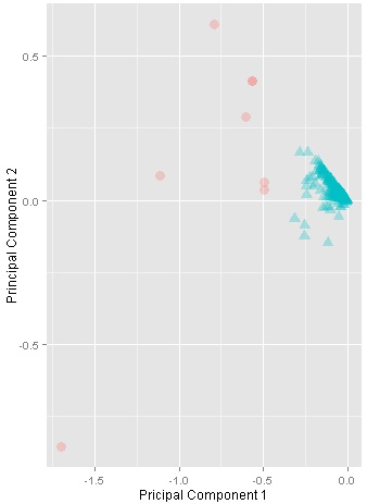
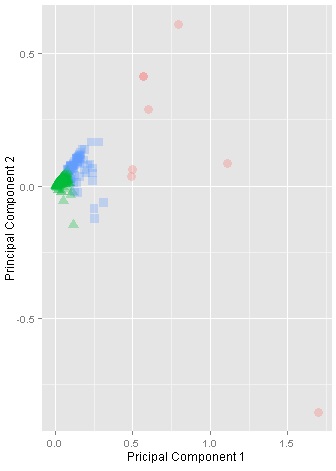
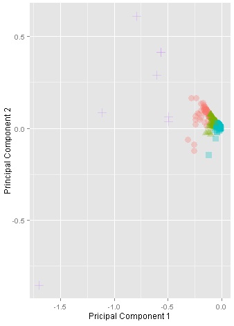
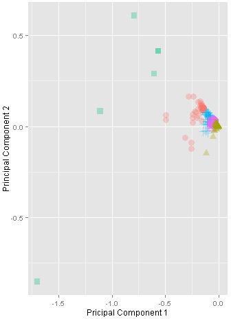
To provide a further visual explanation, the clusters were projected into two dimensions using the Principal Component Analysis (PCA), as in Figure 2. Each sub-figure in Figure 2 represents the output of a single clustering experiment using a different number of clusters (K). Initially with K=2, the output indicated a promising tendency of clusters, where the data space is obviously separated into two big clusters. Similarly for K=3, and K=4, the clusters are still well-separated. However, the clusters started to be less coherent when K=5. Thus, it was eventually decided to choose K=4.
The clustering experiments were conducted using the Azure ML Studio, which provides a flexibly scalable cloud-based environment for ML. Furthermore, the Azure ML Studio supports Python and R scripting as well. The cluster visualisations were produced using R-scripts with the ggplot package (Wickham 2009).
K=2 |
K=3 |
K=4 |
K=5 |
Figure 2: Visualisation of clusters with K ranging from 2 to 5. The clusters are projected based on the principal components.
8. Exploring Clusters
Now let’s explore the clusters in an attempt to reveal interesting correlations or insights. First, Figure 3 shows the proportions of data points (i.e. supercomputers) within every cluster. It is obvious that there is a pronounced variation. For example, Cluster3 contains more than 60% of the Top500 list, while Cluster4 represents only about 2%.
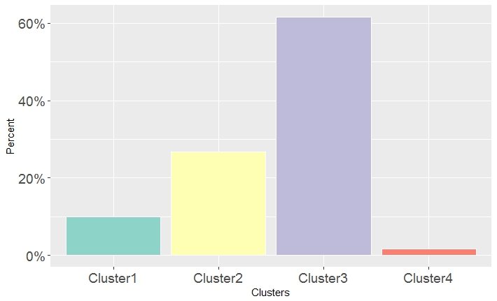
Figure 3: The percentages of data points within clusters.
Figure 4 and Figure 5 plot the number of cores and Rmax against the four clusters respectively. It can be noticed that Cluster4 included the most powerful supercomputers in this regard. It also interesting to spot that “flying-away“ outlier, which represents the supercomputer ranked #1, located at the National Supercomputing Center in Wuxi, China. This gap clearly shows how that supercomputer is significantly superior to the whole dataset.
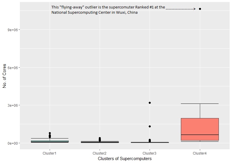
Figure 4: The variation of the number of cores variable within the four clusters of supercomputers.
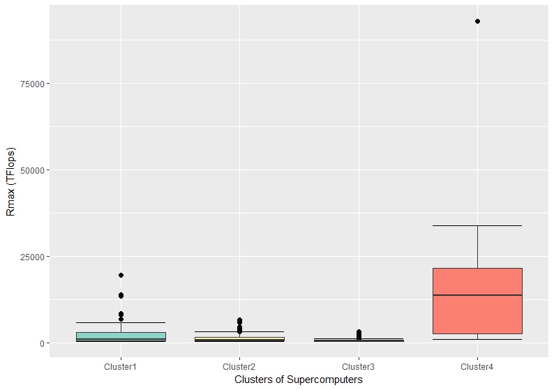
Figure 5: The variation of the Rmax values within the four clusters of supercomputers.
Now, let’s learn more about Cluster4 that obviously represents the category of most powerful supercomputers. Figure 6 plots the segments (e.g. research, government, etc.) associated with Cluster4 supercomputers. The research-oriented segment clearly dominates that cluster.
Furthermore, Figure 6 shows how this cluster is geographically distributed worldwide. It is interesting that the Cluster4 supercomputers are only located in China, Japan, and US. You may be wondering: why the Piz Daint supercomputer (ranked #3) was not included in Cluster4? When I went back to the Top500 list, I found out that the Piz Daint actually has fewer cores than other lower ranked supercomputers in the list. For instance, the Sequoia supercomputer (ranked #5) has more than 1.5M cores compared to about 360K cores of the Piz Daint. However, the Piz Daint has higher Rmax and Rpeak. I am not aware of the process of evaluating and ranking supercomputers, but the noteworthy point to mention here is that this grouping was purely predicated on a data-driven perspective, and considering the expert’s viewpoint should add further concerns.
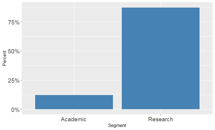
Figure 6: The variation of segments within Cluster4.
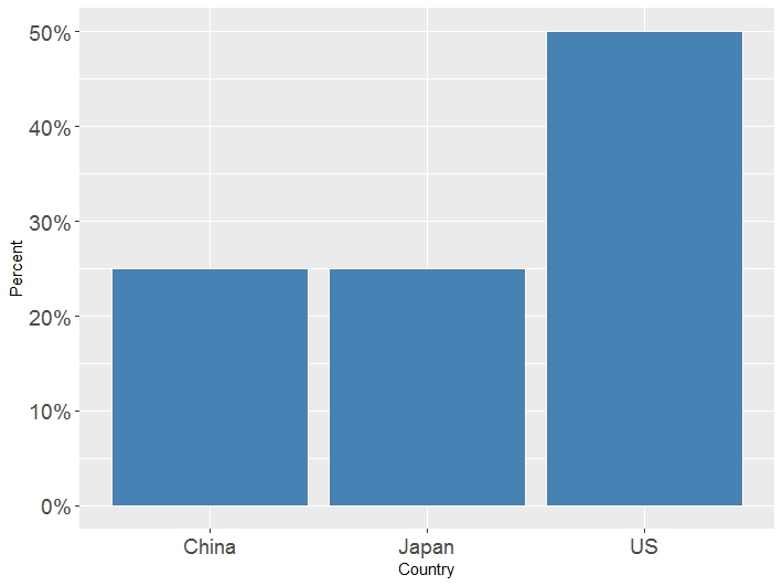
Figure 7: The geographic distribution of Cluster4 supercomputers.
9. Closing Thought
Data clustering is an effective method for exploring data without making any prior assumptions. I believe that the Top500 list can be viewed differently with the suggested clusters. Exploring the clusters themselves can raise further interesting questions. This post is just the kick-off for further interesting ML or visualisation work. For this reason, I have made the experiment accessible through the Azure ML studio via:
https://gallery.cortanaintelligence.com/Experiment/Top500-Supercomputers-Clustering
References
Jain, A. K. (2010). Data Clustering: 50 Years beyond K-means. Pattern recognition letters, 31(8), 651-666.
Sammut, C., & Webb, G. I. (Eds.). (2011). Encyclopedia of Machine Learning. Springer Science & Business Media.
Wickham, H., 2009. ggplot2: Elegant Graphics for Data Dnalysis. Springer Science & Business Media.

Leave a Reply