Optimizing Fault Tolerance for HPC applications with Lossy Compression

Introduction

Hello everyone, welcome to my second blog post for the SoHPC 2021! I hope you are fine and enjoying the summer. It’s been a while since my first post so I will try to briefly inform you about what I have been working on for the past few weeks. For starters, I will introduce the concept of fault tolerance and the checkpoint-restart method. Then, I will explain lossy compression’s role in accelerating said method, which is the goal of my work. Enjoy!

The Need for Fault Tolerance

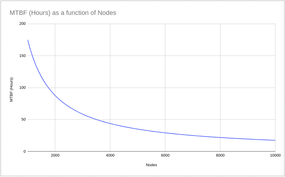
Current HPC platforms, consisting of thousands or even millions of processing cores, are incredibly complex. As a result, failures become inescapable. There are many types of failures depending on whether they affect one or several nodes, and whether they are caused by a software or a hardware issue, or by a third factor, but this digresses from this blog post’s scope. The mean time between failures (MTBF) of a large-scale HPC system is about a day. This means that approximately once a day the system faces a failure. Of course, all processes running during the failure will be killed and their data will be lost. This can be devastating on large-scale applications such as complex numerical simulations which may execute for days, weeks, or even months. Also, while HPC systems increase in scale (see exascale systems), MPBF decreases rapidly, creating many problems. Therefore, the development of Fault Tolerance mechanisms is necessary to be able to continue improving supercomputers’ performance.

Checkpoint/Restart Method

Until this moment, the most common Fault Tolerance method is Checkpoint/Restart. Specifically, an application stores its progress (i.e. the important data) periodically during execution, so that it can restore said data when a failure occurs. Typically the data is stored at the parallel file system (PFS). The disadvantage of this method is that in large-scale applications there is an enormous number of data to be stored, and due to the file system’s bandwidth restrictions there is a high risk of creating a bottleneck and dramatically increase the processing time.

To fight such limitations, certain mechanisms have been developed in order to minimize the data which is written to the PFS, easing the file system’s work. Some of those mechanisms are listed below:

• Multilevel checkpointing. This method uses different levels of checkpointing, exploiting the memory hierarchy. This way fewer checkpoints are stored at the PFS, while the others are stored locally on the nodes.
• Differential checkpointing. This method instead of storing all the data in every checkpoint, changes only the parts of the already stored checkpoint which have been changed, decreasing the number of data that need to be written at the PFS.
• Compressed checkpoints. This method compresses the checkpoints before storing them, again decreasing the number of the stored data. Usually lossless compression isn’t effective since it doesn’t perform a large reduction on the data size. Lossy compression, on the other hand, is very promissing and will be tested during our project.

FTI: Fault Tolerance Interface Library

Our project is based on FTI, a library made to implement four levels of Fault Tolerance, for C/C++ and FORTRAN applications. The first level stores each node’s data to local SSD’s. The second level uses adjacent checkpointing, namely pairing the nodes and storing a node’s data to both itself and its neighbor. This level reduces the possibility of losing the data since for that to happen two nodes of the same pair must die. The third level uses Reed-Solomon encoding, which makes sure that if we lose less than half of our nodes, doesn’t matter which, we can still restore our data. And the fourth and last level stores the data at the PFS. The goal of this implementation is that since the first three levels cover a large variety of failures, we can minimize the fourth-level checkpoints. Also, a differential checkpointing mechanism is implemented at the fourth level of FTI.

Lossy Compression’s Role

At Wikipedia, lossy compression is defined as the class of data encoding methods that uses inexact approximations and partial data discarding to represent the content. Namely, it’s a category of compression algorithms that do not store all the information of the compressed data, but a good approximation of it. The main advantage of lossy compression is that its error tolerance is a variable. Thus we can adjust the compression’s error tolerance to the accuracy of the application. While the error tolerance is lower than the application’s accuracy the application’s results remain correct. For higher error tolerances, we can achieve higher compression rates and increased efficiency. My job is to implement and test lossy compression in the FTI, using the lossy compression library zfp (by Peter Lindstrom, LLNL). After that, we will compare my results with the ones from my partner’s implementation of precision-based differential checkpointing, and gain conclusions.

A Quiz for You!

At the end of this blog post, I have a quiz to challenge you! Which of the aforementioned methods do you think is more efficient in decreasing the bottleneck of HPC applications and why? Multilevel checkpointing, Differential checkpointing, or Compressing the checkpoints? Provide your answers in the comments, and don’t forget to explain your thoughts! No answer is wrong, so don’t be afraid!

Talk to you soon!

Thanos