CESM – Modeling Earth Future Climate

Following the previous post, it is clear why climate modeling is performed using computers. The amount of data and computational needs of climate simulations can be significant, so supercomputers are extensively used to perform the task. In fact, THE strongest supercomputers do climate modeling.

Climate simulations are categorized into two main groups:

1. Operational Forecasting – weekly weather reports or short-term forecast (up to 2 weeks).
2. Climate Research – studying long-term phenomena or developing more sophisticated models.

Respectively, two main software packages are being used for such purposes:

1. WRF (The Weather Research & Forecasting Model)
2. CESM (Community Earth System Model)

In contrast to WRF, CESM is a pure research simulation tool, and is the tool of  interest to us during the project.

Main Challenges

Climate modeling will always seek for more compute power, for several reasons:

• Increased resolution – Detailed simulations
• Accurate physics – Additional physical-chemical processes can be introduced, closer to reality
• Frequent/longer forecasts – Performing more often and for longer periods of time

The target of our project is to introduce GPGPU acceleration into CESM, which in turn will enable more simulations to be performed with higher accuracy.

Global Warming

It is a hot topic nowadays, for good reasons. Notably we see radical variations in weather, but still not completely understood or attributed to a specific natural source.

The thesis being investigated by the local climate research group here at NBI is the affect of ocean states on global warming. Surprising, but yes, a research field called oceanography and closely coupled with atmospheric research. In reality, ice melting at the poles occurs faster than any model predicts, and we would like to know why it is biased. A bit more on that later.

CESM is being used by the IPCC panel to produce climate analysis for the next years, whether it effect air pollution regulation etc. the significance of this model cannot be overestimated.

CESM

This year, CESM (of where there are various generations) celebrates its 30th birthday. Started back in 1983 as an effort by NCAR, it was a basic model for climate research. Over the course of many years it was extended to include more sophisticated physical models until the final form used today.

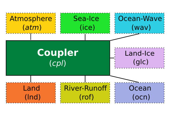
CESM is a coupled model, which means that in order to predict climate states it takes into account contributions from 7 geophysical sources: atmosphere, land, ocean, sea-ice, land-ice, river runoff and ocean wave. Each component with its own physical processes.
WRF for example is based primarily on atmospheric processes, users can add other “plugins” if necessary, but mostly for research and not weekly forecasts.

Baking the Climate Cake

In fact, each component is completely independent of the others, both in runtime (they do not interact directly) and software. For example, the ocean component (ocn) is based on a package called POP2 (Parallel Ocean Program), developed by Los Alamos National Laboratory with slight modifications, and the same holds for others. It is used to simulate processes in the ocean at different depth. How cool is that?!

Using all these sources, how climate is finally formed? It is the role of the coupler, a special component of its own that communicates with each of these geophysical components during time steps, collects data, integrates and updates the model accordingly.

Figure 1: CESM – High Level Component Diagram.
The coupler is in the middle and communicates with all other components through specific channel. Each component is also presented with the shortened form expressed in the system.

Up to this point, you may get an understanding of how complex such a system can be, scientifically and technically. The stress it can put on distributed systems (exchanging so much data) is also very high.

CESM serves as a complete and very flexible research tool, allowing scientific users change parameters regarding physics, but also tune operational layout, like the amount of MPI processes (PE, tasks) given to each component.

Some of the parameters that greatly affect performance are:
Resolution – Dividing Earth into a grid of points, simulations can operate where the spacing is 100 km, 300 km or others. Yes, this is far more crude than the example given in the previous post. For this reason, the model cannot predict different kinds of clouds. And the reasons are…

Prediction Period – How long we would like to predict forward or to the past? CESM is used to predict tens, hundreds or even thousands of years ahead! Not just several days, so a fine resolution model is luxury.

Coupling Frequency – Normally, components exchange data every 12 or 24 hours. It is a lot for some effects to be invisible to the model, like tidal. Increasing coupling means more data transfer and more often.

And we got to the point: it is assumed, that since CESM is configured to perform coupling every 12 hours or more, it underestimates the effect of Near-Inertial Waves on climate. Changing the frequency to 1-2 hours suddenly makes the model more accurate and close to observations.

Architecture

CESM is built in a very modular way, written in FORTRAN (as all climate modeling or geophysics code) and consists of nearly 1.4 million lines of pure FORTRAN code (comments included, configuration excluded).

Each physical component among the ones described above is standalone and obeys a standard interface for initialization, runtime and finalization.

The coupler is the principal component that coordinates and synchronizes components while running. Since CESM uses MPI to communicate in clusters, the coupler also performs the task of designating MPI processes (PEs or tasks) to a component.
Using the configuration, a user can define how many processes should be allocated by a specific setup for each component.

Note that there is no requirement for components to be given equal amount of processes. In fact, some components are heavier to compute than other, or can become intensive based on parameter selection or resolution (atmosphere to the extent). Balancing can be achieved by setting a different amount of processes and the user is responsible for tuning that number to achieve best performance.

To add complexity, the latest version introduced a capability for processes to change roles while running. For example, if the coupler needs to collect data from all components and perform some heavy arithmetic stage etc. it can steal a component’s process to perform that task, and then loan it back.

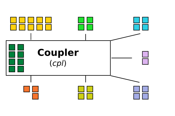
Figure 2: CESM – Component Level.
MPI processes are allocated for each component. There is no requirement that allocation be equal between components. Color scheme was kept for each component.

Component Isolation
To achieve runtime isolation between components, each one is given a unique MPI communicator. Processes allocated for that component use that communicator to exchange data with each other, but cannot with the outside world.

Management wise, a root process is also assigned from each component to allow communication with the coupler. This is the link to the outside world.

Why is all this interesting?

CESM is an example of a unique kind of fascinating systems, very complex and very important. During the course of the project, we came into several architecture considerations of how to integrate GPGPU support using OpenCL to CESM, both for specific algorithms and in general system-wide.

More on that in the next (and almost last) post from Copenhagen.