How to Simulate an Earthquake

It goes without saying that the physics of an earthquake is complicated. This, in combination with the complex structure of the earth’s crust, makes the effects of earthquakes difficult to predict. Luckily, high performance computing and numerical models are the perfect tools to simulate complex earthquake scenarios!
In my first blog post I briefly mentioned that I would work on this project – an HPC wave propagation solver called SEM3D. This software is developed at my host institution and efficiently solves the 3D wave-propagation problem using the Spectral Element Method (a type of Finite Element Method) together with a time-stepping algorithm.
So far so good, but how does this actually work? In this blog post, I will try to summarize my first few weeks of learning, and hopefully give a good high-level explanation of how earthquakes can be simulated in an HPC environment!
Note: The Finite Element Method (FEM) is a popular method for solving differential equations numerically by splitting a large domain of interest (such as the earth’s crust) into smaller, simpler elements (for example cubes). The solution to the differential equation is then approximated by simpler equations over the finite elements. In this blog post, I will assume that the reader has some basic knowledge of FEM and numerical methods for solving (partial) differential equations.
Semi-Discretization of the Wave Equation
The wave equation is a time-dependent second-order partial differential equation, meaning that in addition to the spatial variables, one must also take time into account. Anyone that has ever written FEM code is fully aware of the increased implementational efforts required when going from 1D to 2D, or worse, 2D to 3D.
Since we’re already working with a 3D domain (the earth’s crust), we will not treat time as the fourth dimension in our FEM code, but instead, opt for semi-discretization and a time-stepping scheme. This essentially means that we formulate the spatial dimensions of the equation as a FEM-problem, but express time propagation as an ordinary differential equation which can be solved with a simpler numerical time-stepping scheme.
Spectral Element Method
The Spectral Element Method (SEM) is very popular for simulating seismic wave propagation. Unlike the simpler finite difference method, it can handle the complexity of 3D earth models, while (for this problem) offering better spatial discretization, lower calculation costs, and a more straightforward parallel implementation than normal FEM.
SEM and FEM are very similar in many aspects – both, for instance, uses conforming meshes to map the physical grid to a reference element using nodes on the elements and basis functions. These are some of the key features that differ SEM from FEM:
- SEM typically uses higher-degree polynomials for the vector fields, but lower-degree polynomials for the geometry (whereas FEM often uses the same lower-degree polynomials for both)
- The interpolation functions are Legendre polynomials defined in the Gauss-Lobatto-Legendre (GLL) points (see figure).
- SEM typically uses hexahedral elements in combination with the tensor product of 1D basis functions
- For numerical integration, SEM uses the GLL rule instead of Gaussian quadrature. The GLL rule is not exact, but accurate enough.
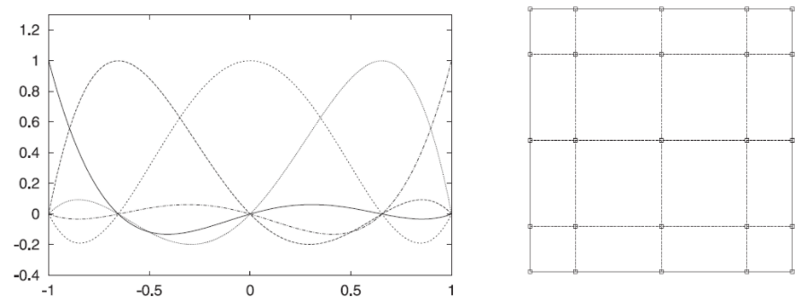
Right: The (n+1)2 Gauss-Lobatto-Legendre points on a 2D face for n=4.
Although it may sound strange to limit the implementation to hexahedra, GLL points, and inexact integration, the combination of the three leads to an enormous benefit: a fully diagonal mass matrix. I really want to emphasize that this simplifies the algorithm and complexity drastically.
Time Stepping
After obtaining the mass and stiffness matrices M and K from the semi-discretization and SEM-formulation, we’re left with a second-order ordinary differential equation Mu”+Ku=F which allows us to propagate over time.
There exist several different time-stepping schemes, most of which are relatively straightforward. SEM3D uses a second-order accurate velocity Newmark scheme in which the velocity (u’) at the next time step is a function of the known velocity and displacement at the previous time step.
Stability
As in all numerical time-stepping schemes, stability (which depends on the time step, dt) is crucial. Since a large time step means less number of iterations and fewer calculations, we want to use the largest possible time step without losing stability. This is where I come in!
The classical CFL condition can be estimated for homogenous materials and structured meshes. When adapted to heterogeneous media, however, the method often becomes unstable. To avoid instabilities, SEM3D uses a safety factor which results in an extremely small time step, making propagation much slower than necessary.
The better alternative, and my job to implement, is an advanced stability condition based on the largest eigenvalue of the matrix M-1K. This advanced stability condition will allow us to calculate the maximum allowed time step without the safety factor, which means that the overall performance of the wave propagation solver will increase significantly!
That’s it for now – hopefully, you have a rough understanding of how seismic wave propagation can be simulated! In my next blog post, I will focus more on my own work and dive deeper into the implementation aspects of the advanced stability condition in Fortran 90 and an HPC environment.

Hi Sara, you have published very well, congratulations 🙂
Thank you Ezgi, I’m happy to hear you enjoyed the post!
Nice explanation!
You mentioned the safety factor that makes the time-stepping very computation intensive. Since you’ll be implementing a different stability condition, does that mean the safety factor in the current code is a rule of a thumb estimate or was it just based on a less fancy condition? And also, how do you know the solution will be stable without this safety factor?
Hi Josip, thank you for showing interest!
The current code still uses the normal CFL-condition (based on the wave speed and time step/element size ratio), but is adapted for the three-dimensional case and polynomial order of the spectral elements. This is of course a less fancy condition, but works perfectly for homogeneous materials and structured meshes. The current “translation” to heterogeneous materials uses the same CFL-condition as the homogeneous case, but applies the lowest local wave speed. This is where instabilities are observed, so the solution is to multiply this “heterogeneous-CFL” with the safety factor. I’m not completely sure how the safety factor is computed – I think it might just be a “hardcoded” value that has shown to ensure stability, but I will have to look into it further. (EDIT: Read the answer from my supervisor Filippo Gatti! 🙂 )
The alternative stability condition (the eigenvalue problem) has been proven theoretically – one of my supervisors have done extensive work on this, so if you’re interested I’d be happy to refer you to some of his papers! With this eigenvalue based stability condition we’re essentially calculating the exact stability limit that also applies to the heterogeneous case, so there is no need to apply an additional safety factor to this.
Hey very nice post! I had so many doubts about SEM, but after reading this I got a really good overview.
Hi
The CFL condition is not “hardcoded” in SEM3D: we can set the “safety factor” on the CFL Condition at each simulation, in order to downscale the time-step an hopefully to avoid instabilities. The CFL condition, however, is computed in a naïve way, as done for regular finite difference schemes. Which is why the choice of the “safety factor” is rather tricky, especially for highly heterogeneous media.