How to visualise a supercomputer

My job is to create a virtual replica of the Marconi 100 supercomputer in which you can visualise data such as the status and temperature of each node. To do this, we first need to know the technical specifications of this machine.

Architecture of Marconi 100

Marconi 100 is a supercomputer created by IBM and launched in 2020. It is composed of 55 racks, 49 used for computing nodes. Each rack has 20 nodes, named using the rack number followed by the node number. For example, node 5 in rack 210 is named r210n05. In turn, each node is composed of 2 CPUs of 16 cores each and 4 GPUs. As a curiosity, with its 32 Pflop/s, it was the ninth largest supercomputer in the world in 2020 and uses the Red Hat Linux distribution as its operating system.

Data to be displayed

The data is contained in an ExamonDB database. Since it is a very large amount of data and we want to facilitate its management, it is stored in a different file for each node, that means 980 files.

The database has information since the supercomputer was started. Data such as the temperatures of both the CPU cores and the GPUs. The power, voltage and memory consumed by each CPU. And one of the most important data for us is the status, which indicates whether the node is working properly or has a problem. A value of 0 means that there are no problems and any other value means that there is a problem.

Creating the 3D visualisation

To create this visualisation we used the VTK (Visualization Toolkit) package for Python and Pandas to handle the data in table form. The CINEMA visualisation team provided me with a 3D model of Marconi 100 which I exported in STL format, as it is very easy to load with VTK’s vtkSTLReader class. (Provigil)

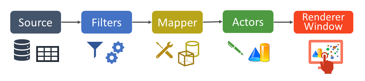
The VTK visualisation pipeline consists of the following parts: Sources, used to read raw data. Filters can then be used to modify, transform and simplify that data. Mappers are responsible for creating tangible objects with the data. And at the end of this pipeline are the Actors, which are responsible for encapsulating these objects in a common interface that has many freely modifiable properties. These Actors are the ones that are passed to our renderer to show them in the scene. In addition to all this, other much more specialised classes can be created that allow us to develop a more interactive environment, among other things. (messinascatering) In my case, I have used this to create keyboard shortcuts that I use to move around the time axis when displaying data.

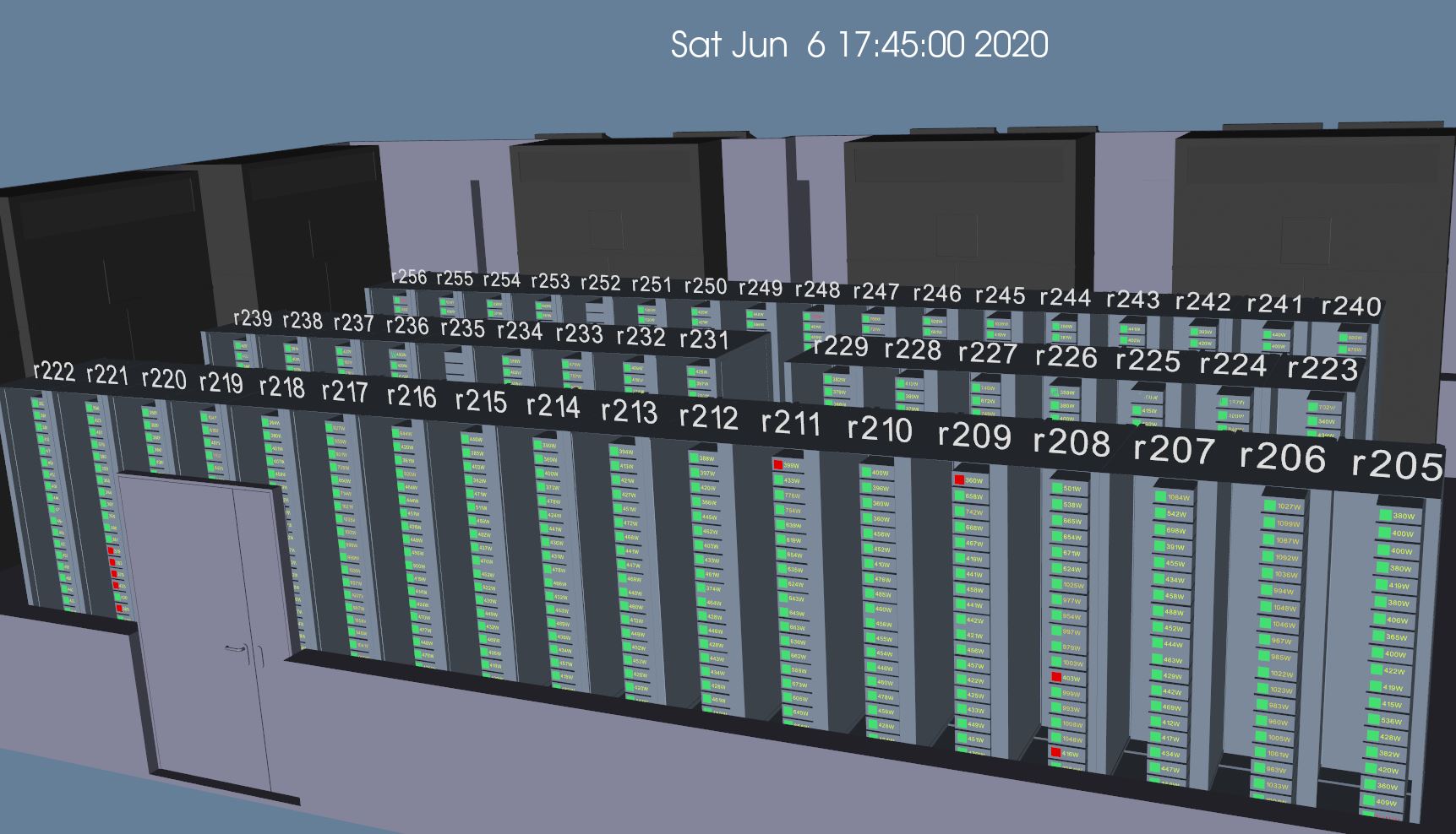
Using all this I have created a first 3D visualisation version of Marconi 100. In this version, I show the status of each node with a coloured plane (green if it is working properly and red otherwise). A text with the consumed power is also shown. And for quicker identification of each node, there is a text with the rack number above it. You can see it in the video below.

The next step is to improve the graphics by adding textures and new data such as core temperatures, where they could be interpolated with a temperature point cloud. In addition, data loading can be improved by parallelising the process.