More on Deep Q networks

The algorithm we talk about here made it to the cover !

It’s time for another blog post apparently! Just as last time, I have decided to fill it with science! This time I will talk mostly about the “Deep Q Network” and the “Stochastic Gradient Descent” algorithm. These are all fairly advanced topics, but I hope to be able to present them in a manner which makes it as comprehensible as possible. Of course, I will provide an update to my project as well.

It’s strongly recommended for most of you that before you keep on reading, if you haven’t already, to read my previous post Artificial Brains for enhancing Crowd Simulations?! and perhaps you’d be interested in my introductory post, about myself and the PRACE Summer of HPC program.

Update on my work

The machine learning part of my project is going very well, and is indeed working as expected. I have several variations of neural network based Q-learning including the Deep Q Network discussed below. In the end, we have replicated most features of the DQN except for the introductory “convolutional layers”. All these layers do, is convert the image of the screen into some representation that is possible for the computer to understand. Depending on the final solution of how we will incorporate the existing simulation, these layers may be put back in.

Our Monte Carlo methods right now are limited to the Stochastic Gradient Descent algorithm and some random sampling during the training phase of the Deep Q Network, as we’ve had some problems with our Monte Carlo Tree Search. This is the Monte Carlo method mentioned in the last post for navigating towards a goal.

It does however look like we have found a way to make it work. However, some implementation details are still required. Where we have before tried to make the tree search work on the scale of individual agents, we have now moved to a larger scale, which means we don’t have the problems we had before with the need of communicating between agents.

Deep Q Network

This network was first introduced in [1] published in the journal Nature, where they managed to play a wide variety of Atari games without having to change a single thing. The Deep Q Network was the first to enable the combination of (deep) neural networks and reinforcement learning in a manner which allows it to be used on the size of problems we work on today. The main new feature added is called “experience replay” and is inspired by a real neurobiological process in our brain. [1]

Compared to the dynamic programming problem of Q-learning, we do “neuro-dynamic programming”, i.e. we replace the function from the dynamic programming problem with a neural network.

In the following video, based on an open source implementation of the Deep Q-Network, we see that in the beginning the agent has no idea what’s going on. However, as time progresses, it not only learns how to control itself, it learns that the best strategy is to create a passage to the back playing area! At the bottom of the page, you can also find links to Deep Minds videos of their implementation.

Basics of Q learning

In the previous post we talked about Markov Decision Processes. Q-learning is really just a specific way of solving MDP’s. It involves a Q-function which assigns a numerical value, the “reward”, for taking a certain action $a$ in a state $s$ . By keeping track of tuples of information of the form $<s, a, R>$ , i.e the state, action taken and reward, we can construct a so called (action) policy (function).

A policy is a rule which tells you that in a certain state you take some action. We are usually interested in the optimal policy which gives us the best course of action. A simple solution, but not very applicable in real world situations, is explicitly storing a table specifying which action to take. In the case of a tabular approach, we simply update the table whenever we receive a better reward than the one we already have for the state. In the case of using neural networks, we use the stochastic gradient descent algorithm discussed below, together with the reward, to guide our policy function towards the optimal policy.

An important thing to mention here is that it is important that we don’t always follow the optimal policy, as this would lead to us not obtaining new information about our Q-function. Therefore, every now and then, we take some random action instead of the one given by the optimal policy. A smart thing to do is to do this almost all the time in the beginning, but reduce it over time. We can perhaps see the analogy to growing up. Children often do things we, as adults, know not to do, this way they learn; by exploring the state space and seeing if they are rewarded or punished.

Experience Replay

During learning, episodes of sensory input and output are stored and later randomly sampled, over and over again to combine previous and new experiences. An episode contains information about which action was taken in a state, and what reward this gave. This technique is also done by the brain’s hippocampus, where recent experiences are being reactivated and processed during rest periods, like sleeping. [1]

Stochastic Gradient Descent

Let’s, for a moment, skip the stochastic part and concentrate on the gradient descent. Imagine you are on a hill and want to get down as quickly as possible, i.e. take the shortest path, having no access to a map or any information about where you might be or the surroundings. Probably, your best bet is to always go in the direction of the steepest descent.

In the case of machine learning, we are in a bit more abstract world, and would like not to get to the ground, but find the (mathematical) function¹ that most closely resembles our data. One way of doing so is minimising the so called $L^2$ norm, which is the “straight forward” generalisation of Pythagoras Theorem, $a^2 + b^2 = c^2$ , from points in the plane to distance between functions. How this works can be seen, I think, quite easily from the gif below. Simply let $x=a$ and $y=b$ where x and y are the length of the catheti along the x- and y-axes, respectively. Then just bend your mind for a while!

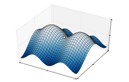
Imagine being somewhere on this graph. You want to get down as fast as possible, so always head in the direction of the steepest descent. There is a risk of hitting a local minimum (white dot). However, this can easily be overcome by having a look around.

Taylor series approximation for the real exponential function

The Taylor series approximation for the exponential function.

This gives us a a direction to go towards! One problem in the case of very high dimensional functions is that this can be very time consuming. Therefore, we often use Stochastic Gradient Descent (SGD) instead, which updates only one, or a few, dimensions at a time. This is done randomly, hence stochastic in the name.

How on earth does this relate to the image of the neural net I showed last time, you may ask? Well, this is where the magic that is neural nets comes in. As far as I can see on the internet, no one has explained this in a easy to understand fashion; in partiuclar it would require a very long explanation on exactly what the networks do. You can try to visualise some connection between the dimension of the function and the neurons (the circles in last weeks picture).

¹ – These functions might not be as simple as most people are used too. For a starter, in school, we meet functions in 2 dimensions and of the form $y = f(x)$ . The functions I’m talking about will often have tens of millions of dimensions.

Well, that’s it. The actual algorithm is presented below, and will not be explained. I refer to the original authors’ paper.

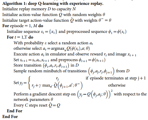
Deep Q-learning algorithm. This version deals with processing images, hence the mention of images. Not intended to be understood by the vast majority, but included for completeness for those who can.

References

[1] DeepMind Nature Paper https://storage.googleapis.com/deepmind-media/dqn/DQNNaturePaper.pdf

Videos from Deepminds original implementation:
http://www.nature.com/nature/journal/v518/n7540/fig_tab/nature14236_SV1.html

http://www.nature.com/nature/journal/v518/n7540/fig_tab/nature14236_SV2.html

Image is from the cover of Nature, issue 518, Cover illustration: Max Cant /Google DeepMind

More on Deep Q networks

Update on my work