Puzzle-Error-Puzzle-Error-Run

One step forward, two steps back. The reality in the world of programming: At one moment you are making progress, as easily and efficiently as standing your dominoes end-to-end and then you just nudge your first domino and hundreds of dominoes follow by themselves, and at another moment you try to fix a problem for three days, where you are not even sure if there is anything there to fix at all.

After the Training week I started with the system set ups on the UK national Supercomputer: ARCHER2, required for the MPAS atmosphere model runs. This has entailed, installing new modules, setting up directories for the libraries, like netCDF, or HDF5 for a parallel environment and preparing the Makefile for the MPAS installation. A lot of Errors came up, but I persevered on, and so I was able to go on to the next step: preparing MPAS for small runs, which means taking a small input mesh and a short simulation time. In principle there are two steps, that need to be done for this, the first, is to create from a mesh and from the input parameters, an initial condition file. And the second is, based on the initial file you can then run the simulation itself. To accomplish this well, and also with a view to future model runs, you try to write scripts for everything where it is possible. So of course, you need a job script, where you tell the cluster the details, like on how many nodes you like to run your simulation on, how and where the output should be stored, but especially also the run command itself. But it is also very useful to write a pre-processing, a run and a data visualization script, because it would be very time consuming to do this for every run ‘by hand’. In the previous week I was concentrated on the visualization script, which I decided to write in Python. Because on the one hand, Python is a widely used and easy to handle, and the other hand, it provides an interface to the netCDF library.

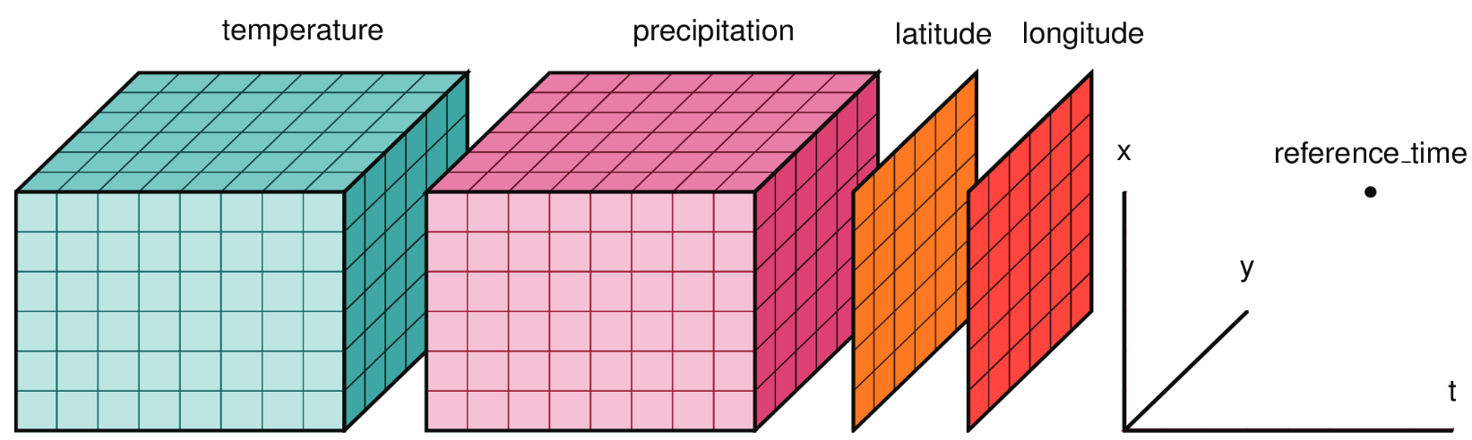
This is important, because the output of the MPAS runs are netCDF files, where you have the 3d mesh coordinates, and physical relevant output parameters, like temperature at different pressures, wind velocity, vorticity etc. stored in n-dimensional arrays.

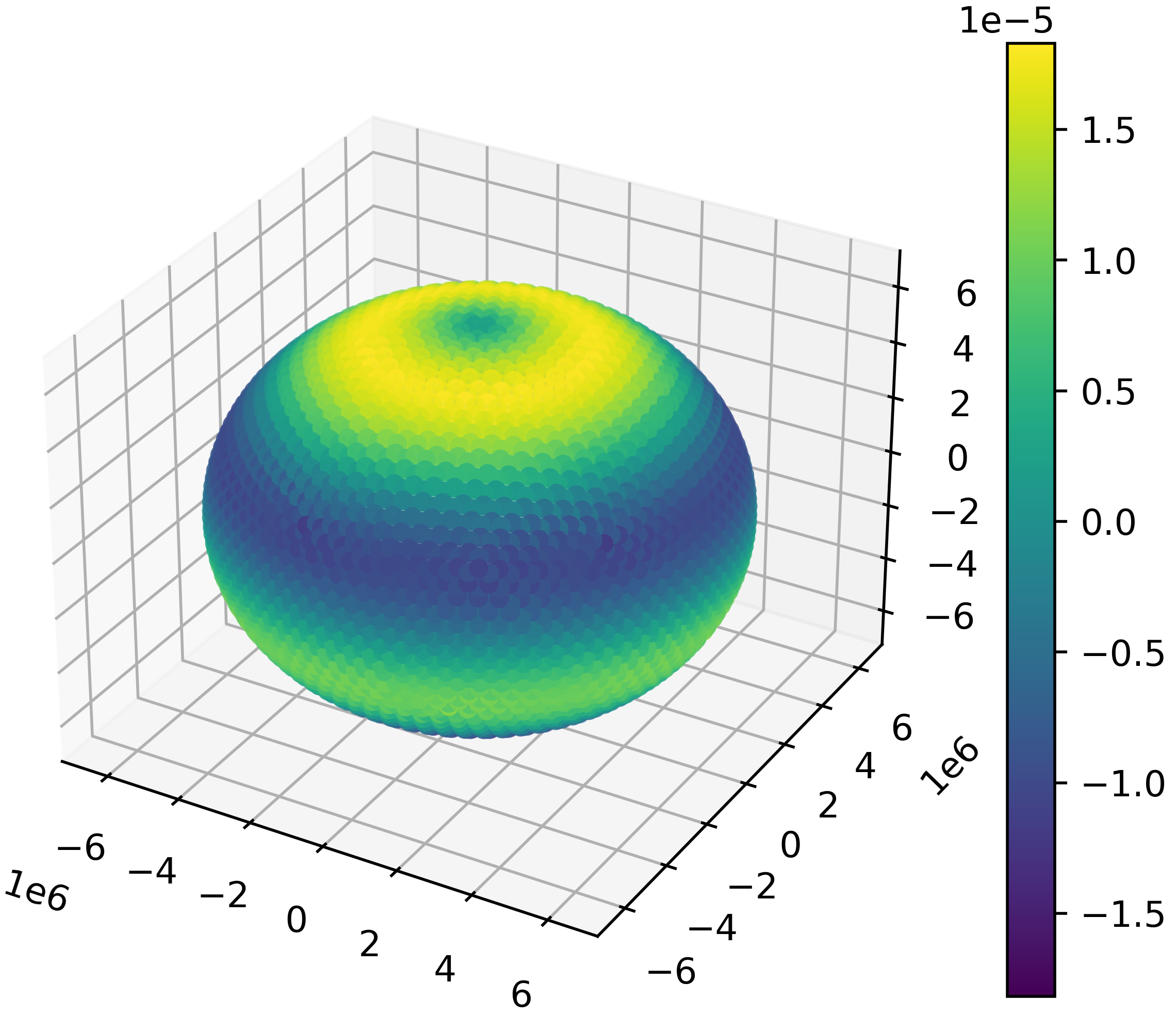
In my visualization script I load these Datasets, assign them to one dimensional Python arrays, and I am then able to plot them with matplotlib, like every other array. Of course, this is only one part of the story, the further step is connecting the visualisation script to the pre-processing and running script and that you enable the script in a way, that you just have to type in which parameters you want to have plotted and the rest is automated.

Before we can visualize any data we have to produce a data set. We structure our test runs into small, medium and large ones. Where small/medium/large runs, are not only characterized by the mesh size of the model run, but also on simulation time and the core count we use for those runs. Additionally how different run parameters and some physical parameters influence the calculation time of our simulations will be investigated, as part of understanding the puzzle of MPAS and computational efficiency on ARCHER2.

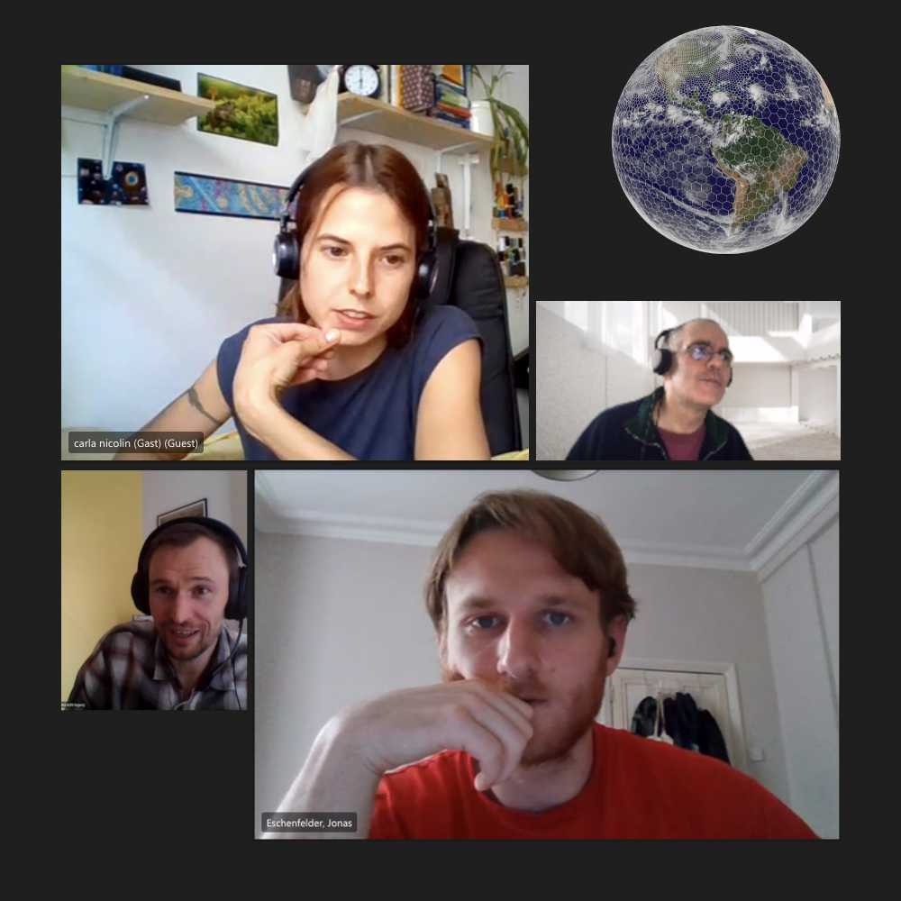
Looking forward spending this summer together with Jonas Eschenfelder (check out also his Blog post on PRACE Summer of HPC website: ‘First steps with a big impact’), Dr. Evgenij Belikov and Dr. Mario Antonioletti on the Project: ‘Investigating Scalability and Performance of MPAS Atmosphere Model’ and report to you at least at the end of August about my experiences and results from this captivating project.