The end of the road

In the last blog, we discuss what a CNN is, what “flavor” of CNN we were using, and how we solved the issue of the cost function adapting the cosine similarity to work on our problem. Now it’s time to show how all of this work out in the training process and what outcome we archived.

The training process

To train the neural network we needed to structure the data in a way that is easy for the network to go through and understand. For that, we created a dataset with the normalized labels of the galaxies and the corresponding images. Once we have done that, we need to initialize the network with values for all the parameters. When the network has weights and biases we can feed data through it, see the results (at first all are gonna be random guesses), and compute our fancy cost function to see how far we are from the ground truth. When we have the error that we made we can update the network (change the weights, biases and kernels) with our optimizer. We chose the Stochastic gradient descent (SGD) as our backpropagation method.

Improving the dataset quality

As in any scientific process, we didn’t achieve perfect results at the first try. The first training runs were quite a mess. We started using the imagenet pre-trained weights. Then we realize that the images were too similar to each other and imagenet was always predicting the same output for all of them because the network was too stable to learn properly. Then, we changed to a randomly initialize network and the things went better (not by much). After that, we focus on one of the most important things in machine learning, the data. We restricted our dataset to just the galaxies more massive of 10^11 solar masses to have enough quality in our images, that made a significant change in our results.

• 

• 

When 24 CPU’s is not enough

As we advanced in the project, the training runs take longer and longer each time on the CPU cluster. As this is a highly parallelizable task and is based on the perfect operations for a GPU, we moved all the training process to a GPU cluster with 4 Nvidia Volta 100. We went from 5h runs to 27 minutes… Not bad. But this not came without a cost. We needed to adapt our code to work in multiple GPU’s and to be extremely careful with the way we pass our data and update the weights to avoid possible conflicts.

The results

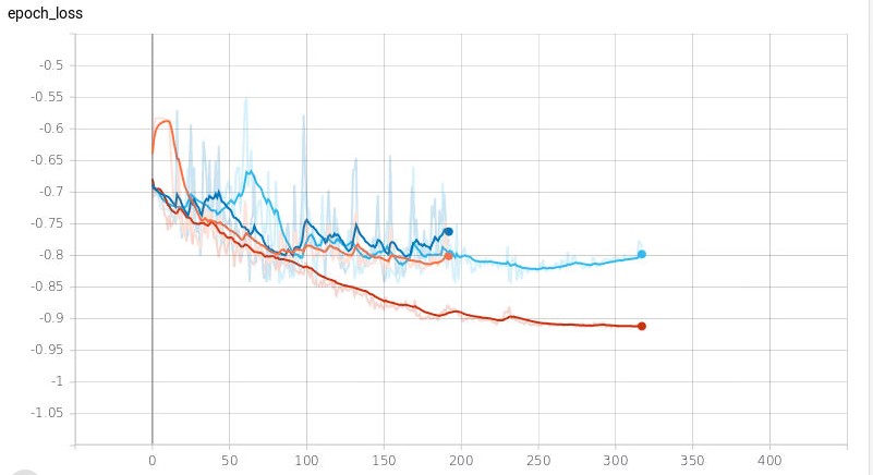
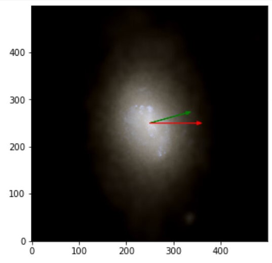
At this point, you may be thinking… Okay, but what did you get ??!! Okay, here comes the results. The metric we used is the adapted cosine similarity function where -1 is a perfect score and 0 is totally off and this is what we find:

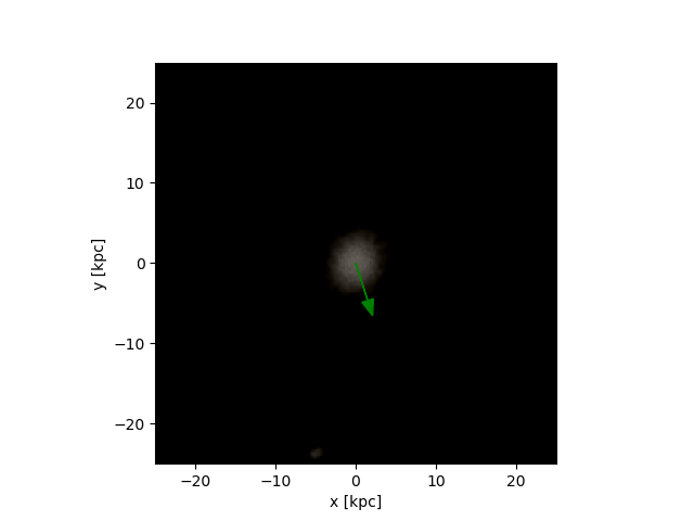
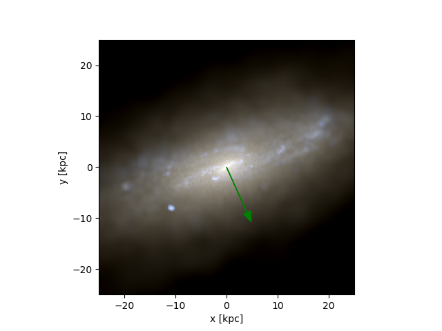
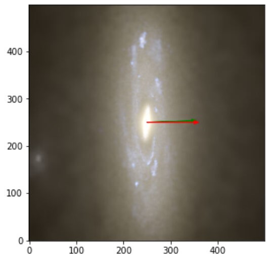
The images obtained with labels and predictions for the validation dataset are:

• 

• 

• 

• 

• 

From there, and armed with all the things I learned in the SoHPC I will be looking for ways to improve this results and take it to another level… This was the end of the road but now I’m in the unexplored, the wild territory where real exploration is made. And thanks to the SoHPC I’m ready to face it.