What is Hamiltonian Monte Carlo?

Generating random variables from an arbitrary distribution is a surprisingly difficult task, and Hamiltonian Monte Carlo (HMC) solves this challenge in an elegant way. Let’s consider a multivariate target distribution ")

Most Markov Chain Monte Carlo (MCMC) methods work by generating the proposals for the next sample (

This simple MCMC method struggles with high-dimensional distributions, as the volume surrounding the typical set is much larger than the volume of the typical set, meaning most propositions are in areas of low density and are therefore rejected. This isn’t very efficient, we can reduce the step-size to increase the acceptance rate, but this causes samples to be highly correlated.
This is where HMC steps in. Each point in the parameter space =-\ln{\pi(\vec{q})}")
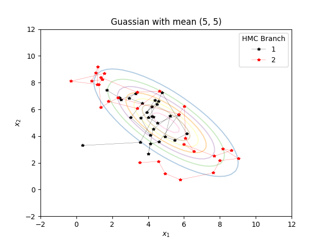
 = \exp(-q_1^2-q_2^2)")
To go from one sample to the next, we give the “particle” a random momentum 
Up until this point, Bruno and I have been working to implement and parallelize this algorithm with the help of our mentor Anton. In the next blog post I’ll talk about how we’ve been using jax, a python module which massively speeds up numpy on CPUs and GPUs.
References
Tom Begley’s Blog Post – Thanks for granting me permission to use the animation above!
M. Betancourt – A Conceptual Introduction to Hamiltonian Monte Carlo
Physics Student @ UoManchester Graduating 2024, with a strong interest in computation and statistics.
