Shallow waters – the waves start to spread
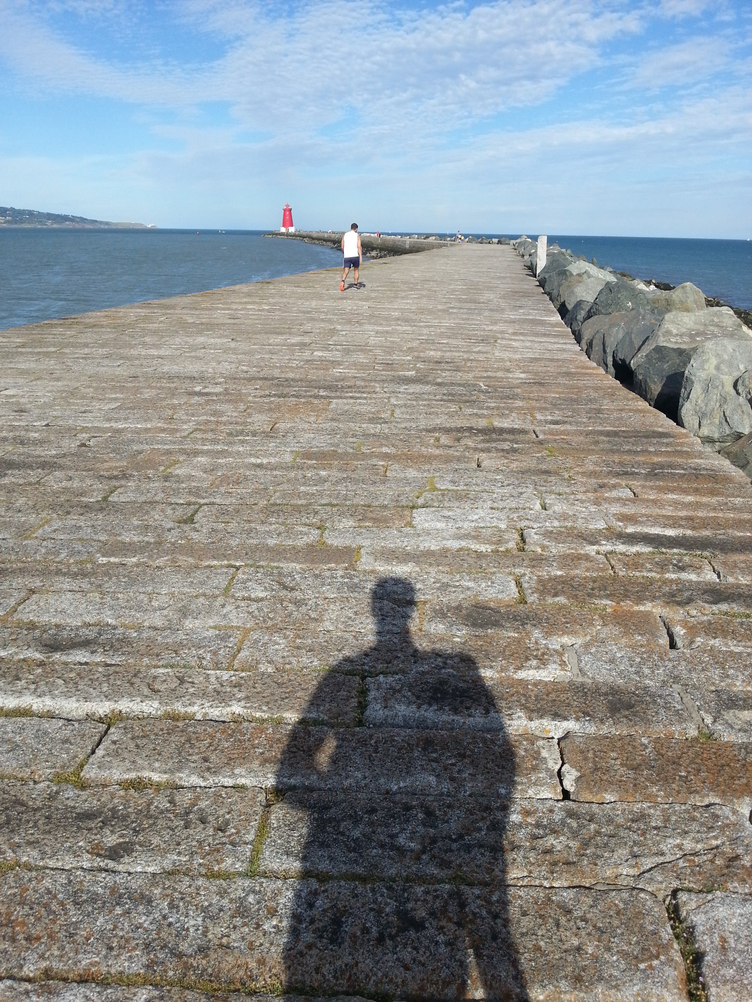
The Great South Wall, Dublin Bay
I started the work on my project by exploring the provided simulation code. This is always a great adventure by its own, studying a code someone else has written before you. To those who never tried it, you definitely should. I must give all the credit to the creator of the original code, for making it nice and tidy, well structured and filled with meaningful comments. The latest one especially made my job significantly easier, and should be awarded by some sort of medal, because comments in code is something you don’t see too often, at least from what I’ve experienced. Thing that was making my progress a bit slower was the programming language used for the code – Fortran. For me, who spent most of the time coding in C++ language, the Fortran syntax was quite confusing and unnecessarily complicated at some points. But I managed to handle this little complication, and learned a new language, which is always a good thing. Also, after some initial struggles, I must also recognise some positives of the language, like an easy array multiplication syntax, without need for any library.
The next step in my work was to paralli, palare, para … Alright, the next step was to learn how to pronounce the word parallelisation properly, and also spell it right. This took me around a week, and yet it’s still not perfect, so I would like to challenge language institutes across the world to come up with a better word for this phenomena.
 Anyway, the next step was to make the code parallel. I used the OpenMP library for this. The library provides a simple framework for letting the code run on multiple cores on one computational node. With my supervisor, we decided to use OpenMP for its simplicity, and also for the fact that the parallelisation (uf …) of the code is only possible over the space domain, and not the time domain. In other words, all threads must synchronise (wait for each other) after each time step of the simulation. Since the space domain is not too big in this case, one processor, equipped with 24 cores is good enough. In simple words, using too many workers for a small job can turn out contra productive.
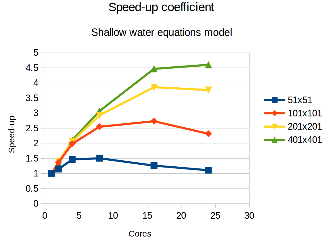
Simulation benchmarking – each curve represents a domain of different size
Once I modified the code using OpenMP library, I was ready for some benchmarking on Fionn. I was provided with an account on this system, so I could run the simulation code on one of the Fionn’s nodes. As stated before, those nodes consist of 24 processing cores. You can see some results of the benchmarking in the attached chart. Naturally, more cores make the code run faster. Using a bigger domain results in higher speed-up, since there is less time (proportionally) spent on the thread synchronisation after an each time step, and more time on an actual work. In general, it’s clear the speed-up is not that big, considering we got only around 5 times faster run time while using 24 cores. This is probably due to the computational domain still not being large enough, and also the parallel implementation might not be the best possible one.
After debugging the parallel version of my code, and benchmarking it on Fionn, I moved to the visualisation part of my project. I started with ParaView, a software frequently used to visualise scientific data. This first required to output the data in some ParaView compatible format. While ParaView supports plenty of different file formats, it can not read the Fortran binary format. First I used the csv format. Csv is nice, tidy, simple, understandable, readable, and works pretty much everywhere. The problem is, it’s also catastrophically slow, to both write and read. So, I moved to the netcdf format, which is a scientific data dedicated file format. It’s way faster to write, and ParaView is able to read it. With the suitable file format prepared, I could start playing around with visualisation methods, displaying height maps, velocity vector fields and 3D surfaces of the shallow water simulation. At the nearby picture, you can see a sample visualisation generated from the simulation output, using 201×201 points grid, with reentrant boundary conditions (i.e. what goes out on one side, comes back on the opposite side). I am still working on the visualisation part, so I will have more material to show at the end of the project.
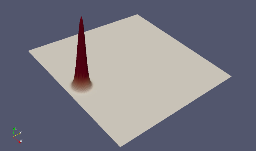
Shallow water simulation – 3D surface plot of the initial state – a Gaussian bump
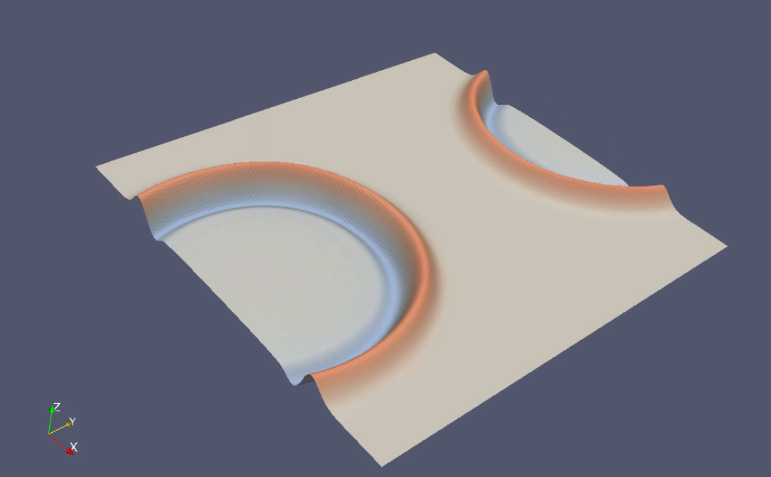
Shallow water simulation – 3D surface plot state after a several thousands of simulation steps
During my free time, I explored a few places around Dublin. It is a very unique place. The place I live at is very close to the night life centre of the city. You basically pass one pub after another, all of them stuffed with people, with even more standing around outside of the pub. During the weekend, those places don’t sleep all night. On the other hand, you can find a large parks full of green, flowers and little lakes, where everyone can get their peaceful relaxing time. Naturally, there are also historical places to see in Dublin.
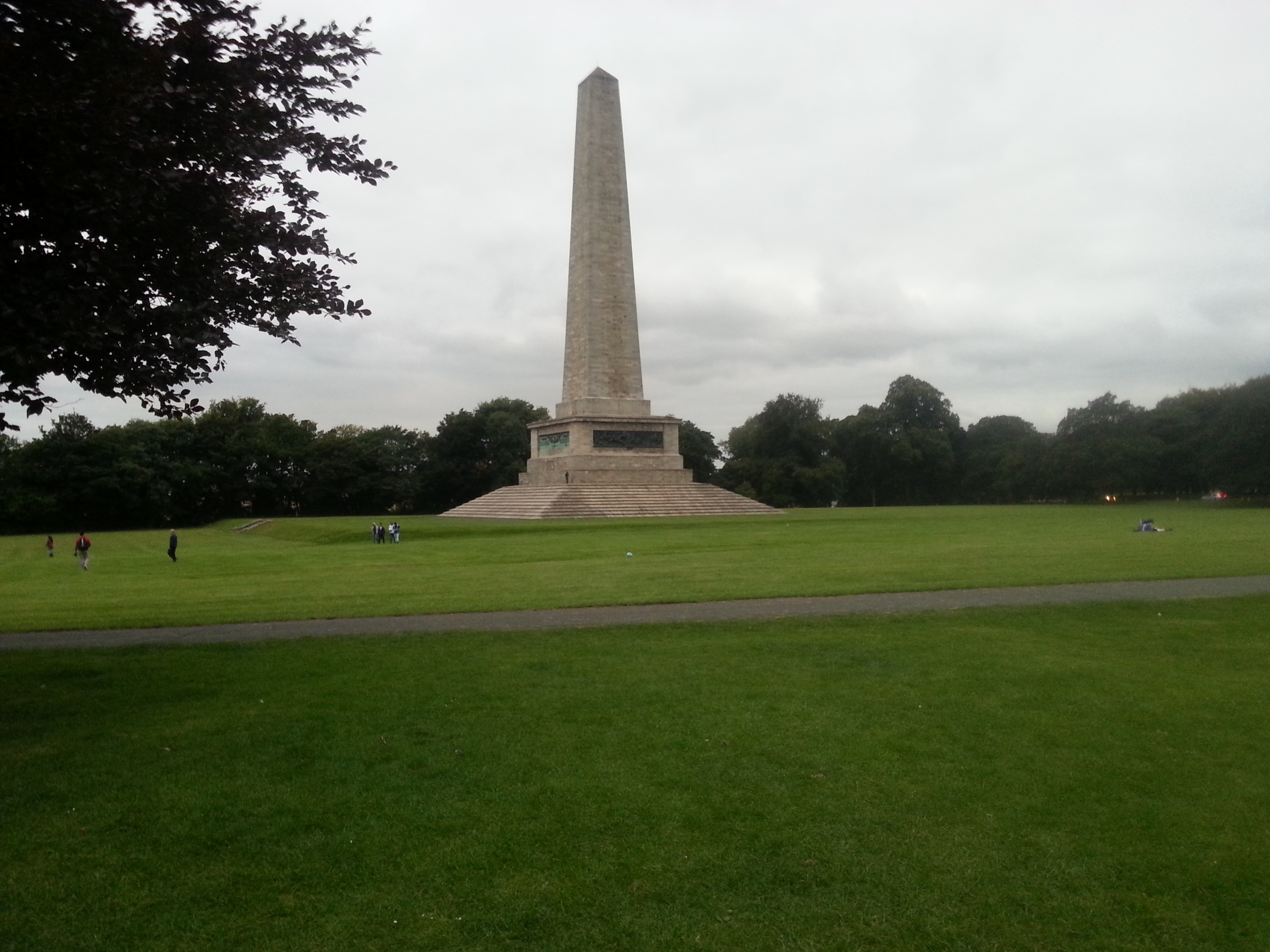
The Wellington Monument
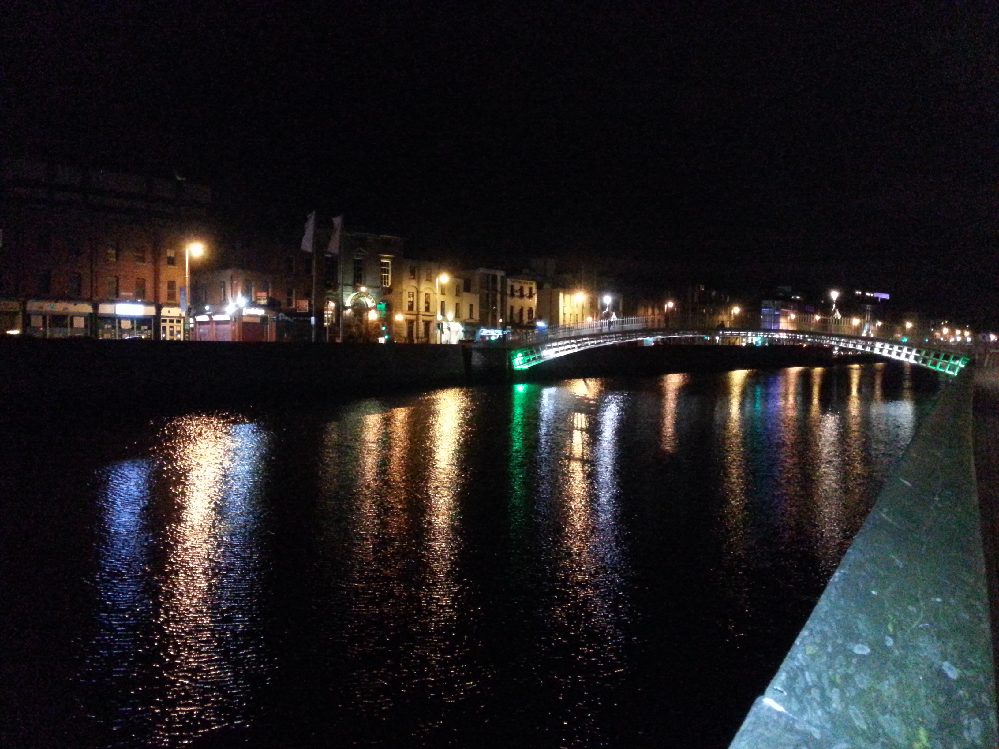
A night in Dublin – a colourful reflections of street lights in the Liffey river
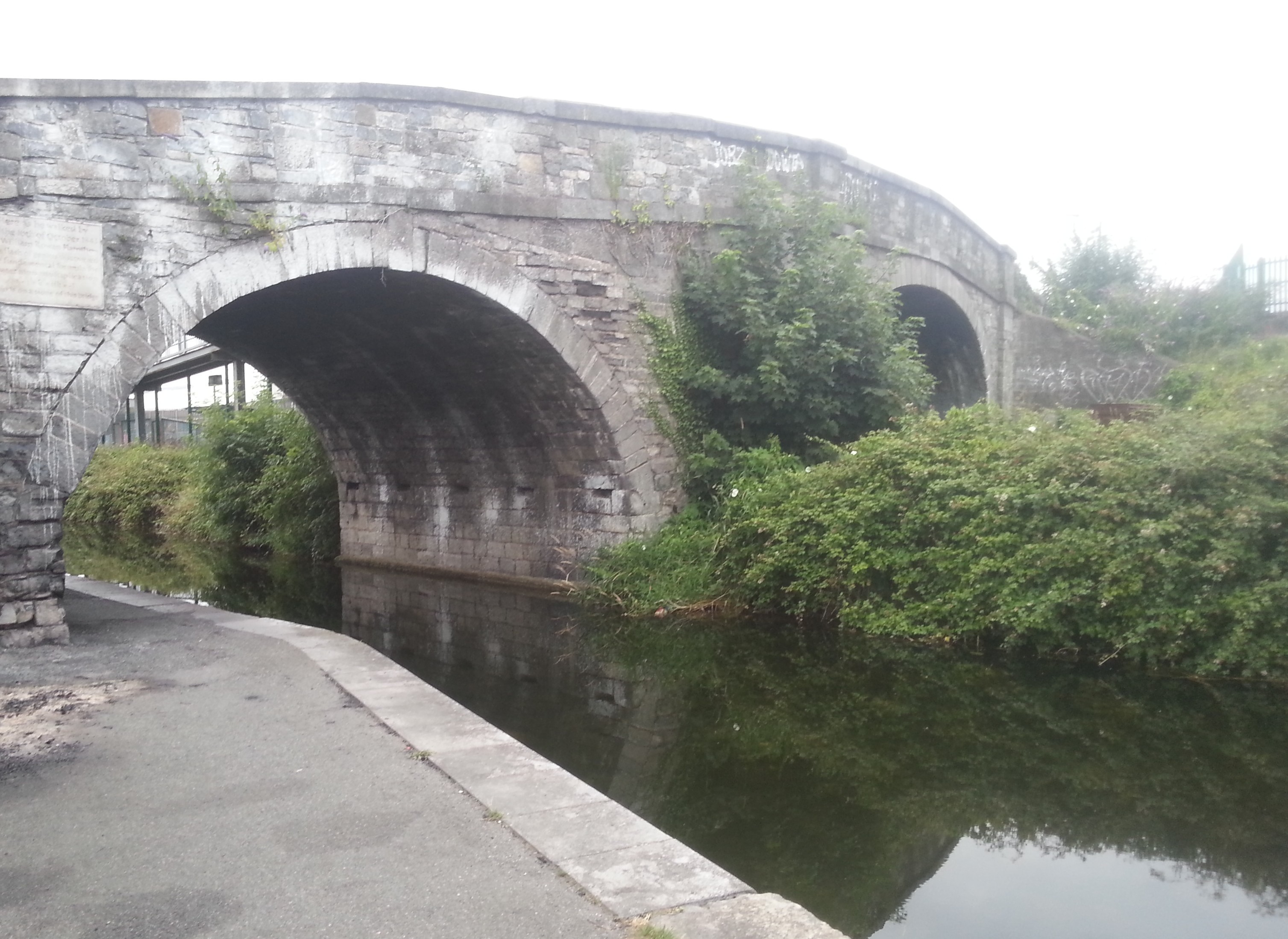
I visited the Wellington Monument, named after the British army field marshal, who defeated Napoleon in 1815 century at Waterloo. Then I went to see a place which has a big importance in the mathematics world – the Broom Bridge. It is the place where, in 1843, mathematician Sir William Rowan Hamilton wrote down his rules for quaternions for the first time.
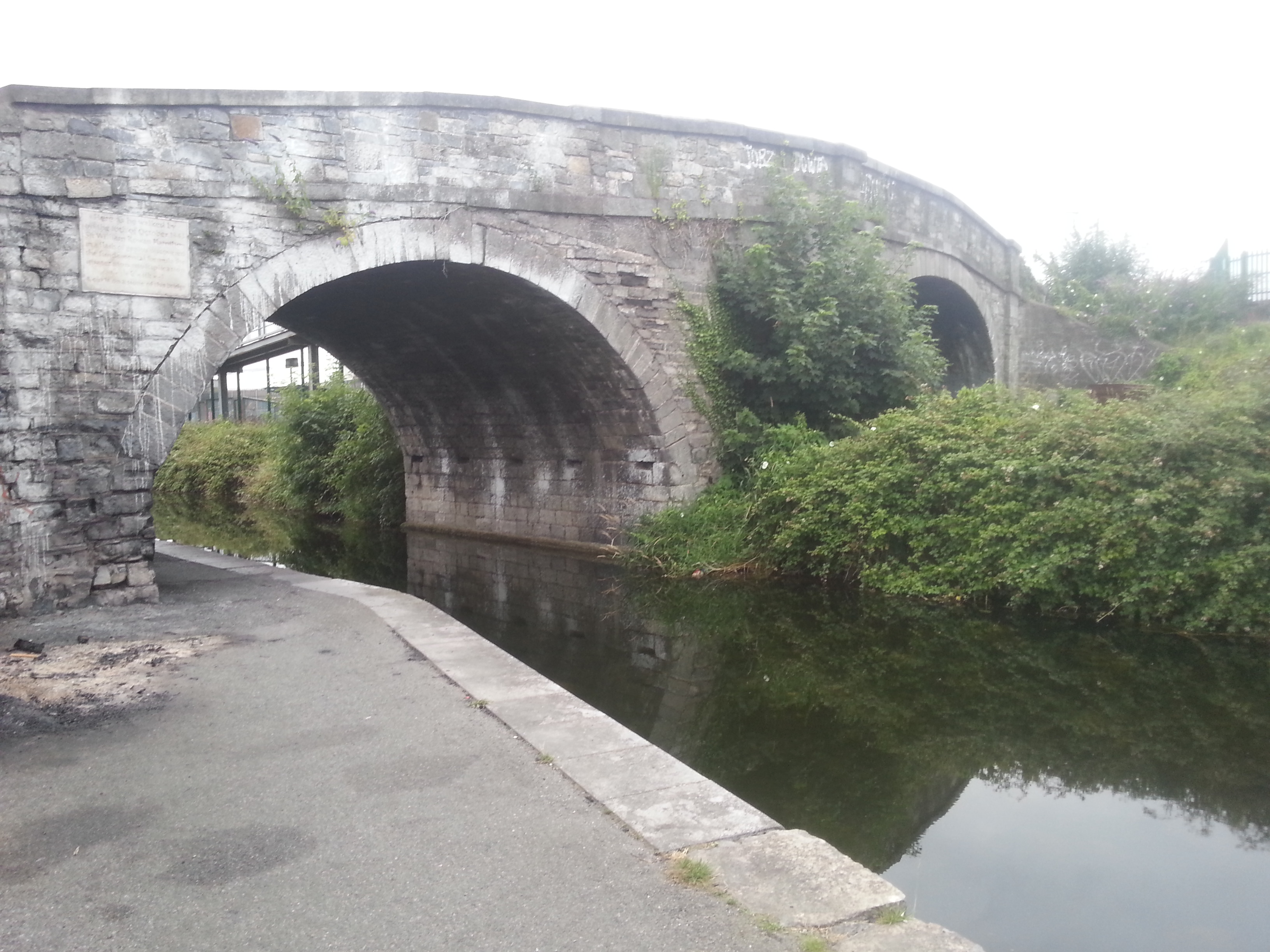
Tne Broom Bridge
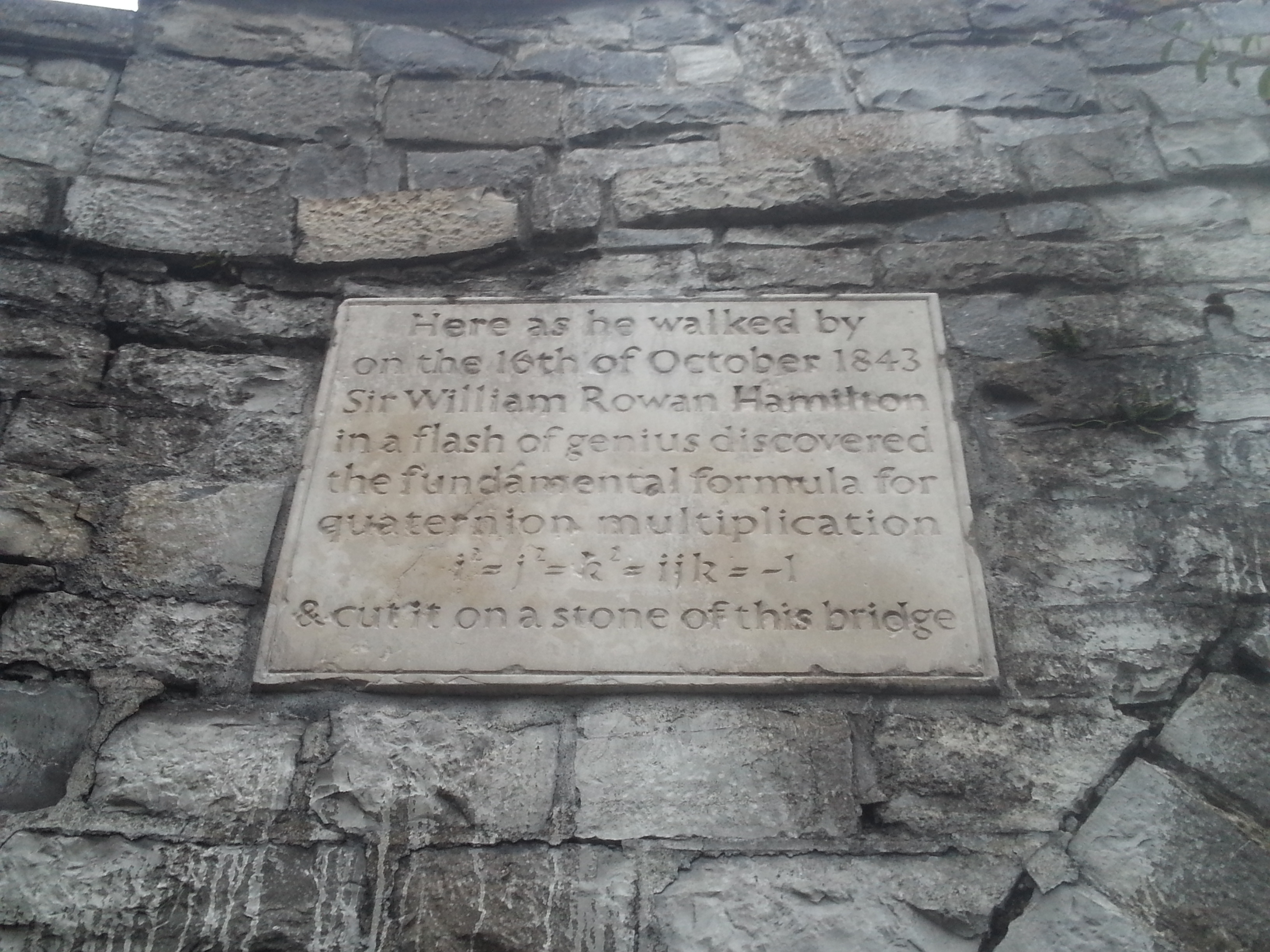
The plaque reminding Sir William Rowan Hamilton, and his set of basic rules for quaternions
