Accelerating physics simulations with data science and vectorization

Last few weeks, it has been a very interesting time here at the Jülich Supercomputing Center. Unfortunately, I only have a bit more than a week to spend on these fascinating topics with the inspiring people here at the center.

Vectorization by hand

In this section I present some of my practical exploration of the vectorization capabilities of GCC (GNU Compiler Collection) and ICC (Intel C/C++ Compiler ) for a small code that performs a simple operation over vectors of data. The most important outcome of this task was to familiarize myself with code vectorization so I will be able to modify and optimize vectorized code in more complex software such as physics simulators.

In the Figure below we can see the performance of the application for different problem sizes and compiler optimization levels. As we can see each time the vector size increases more than a cache level size, then we have a performance overhead because the data need to be fetched from a higher level of the cache hierarchy, which is more expensive to access.

Performance for different problem sizes and GCC compiler optimization levels on a Jureca node.

For the above experiment I did not specify any vectorization intrinsic into the code. I was expecting from GCC to exploit vectorization but it did not. This is the reason that inserting commands from a selection of intrinsics supported by the processor could be a good idea to ensure that the code is vectorized.

Below we can see a similar set of results that compares the performance achieved with and without manual vectorization.

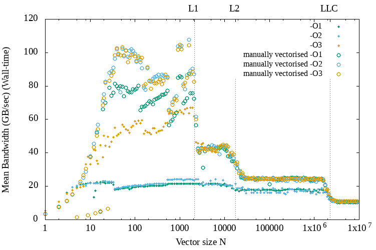
GCC compiler vectorization vs vectorization by hand (FMA intrinsics)

As we can see, at least for the small programs sizes below the L1 cache size manual vectorization almost doubles the performance when using the O3 optimization flag and triples it when using a lower optimization level.

For the Intel compiler though this was not the case. ICC was able to exploit vectorization. Of course, the compiler technology could become very efficient for auto-vectorization in the future and this would be more desired over a code with intrinsics, which can have architecture portability issues. But for HPC applications it can still make sense to continue vectorizing code manually because of the specialized nature of the software and hardware infrastructure.

Accelerating the simulations with online optimization

Simulations of Lattice QCD (Lattice Quantum Chromodynamics) are used to study and calculate properties of strongly interacting matter, as well as the quark-gluon plasma, which are very difficult to explore experimentally due to the extremely high temperatures that are required for these interactions (click here for more). The specific simulator we are trying to optimize is using Quantum Monte Carlo Calculations, which have originally been used for LaticeQCD, to study the electronic properties of carbon nanotubes [1].

My last activity was to help eliminate the simulation time of  the simulator by using data science techniques. The method I will describe in this section is independent to the parallelization and vectorization of the code for fully exploiting the computing resources. The code of the simulator is already parallelised and vectorised, perhaps not optimally, but as we are going to see, some algorithmic decisions can further accelerate their execution.

The simulator uses leapfrog integration to integrate differential equations. The equations that are used for the integration look like recurrence relations, which means each next value is calculated using a previous value. Specifically, the smaller the time difference (Δt), the more accurate the integration is. Δt is inversely proportional to the number of MD (Molecular Dynamics) steps (Nmd) . Therefore, the greater Nmd gets, the more accurate the simulation is but also the more time it takes to finish. If the value of the Nmd is low, the acceptance rate of the new trajectories is too low for getting useful results in reasonable time, even on a supercomputer. If Nmd is too high the acceptance rate is 100% but it introduces a significant time overhead. The goal is to tune this parameter on runtime to select the value that would yield an acceptance rate near 66%.

In computer science, when an algorithm is processing data as soon as they become ready in serial fashion is called an online algorithm. In our case we need such an online algorithm for tuning Nmd because each data point is expensive to produce and we do not have the whole dataset from the beginning. Also, we are not aware of the exact relationship of the acceptance rate with the other parameters, such as the lattice size. We could do an exhaustive exploration of the other parameters but it could take an unreasonable amount of time for the same computing resources. Of course there are shortcuts to creating models when exploring a big design space, but the dynamic approach makes it less complicated and more general for future experiments where new parameters could be added without the knowing the amount of their orthogonality.

The idea is to create a model of the relationship Acceptance Rate versus Nmd each time a new data point comes in and then select the best Nmd for the next run. In the following figure we can see a set of observations from an experiment, as well as the model my (earlier version) auto-tuner can create. It uses the least-squares fitting functionality of the scipy python library to create the model based on a pre-defined equation. As we can see observations have an (almost) sigmoid-like shape and therefore we could fit a function like f(x) = 1/(1+exp(x)).

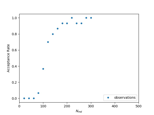
Observations for different number of md steps

The algorithm that scipy uses to fit the data is the Levenberg-Marquardt algorithm. As a user it is very simple to tell the algorithm what parameters need to be found. From high school mathematics we already know that we can shift, stretch or shrink the graph of a function with a set of simple operations.

• If we want to move f(x) to the left by a, we use f(x+a)
• If we want to shrink f(x) by b in the x-axis, we use f(b*x)
• If we want to move f(x) up by c, we use f(x)+c
• If we want to stretch f(x) by d in the y-axis, we use d*f(x)

Since we already know that the acceptance rate ranges from 0 to 1 then we do not need the last two of the above. Then, our model has the form 1/(1+exp((x+a)*b)), which is fast and accurate even if we only add a few points (beginning of the simulations). This example is a bit more simplistic than my actual algorithm.

And here is an animation that shows how the regression is progressing through 40 iterations.

Animation: Least-squares fitting in action

Conclusion

This has been proven useful for our simulator and in a next post I will explain more about the specific algorithm I used for fine tuning the simulations for less runtime.

Regarding the vectorization, I did not have much time for a second task, to further optimize the current implementation, but I learnt a lot during the initial hands-on activity described above and can easily apply it in other problems in the future, as well to identify bottlenecks in performance.

Other activities

I have also had a great time visiting Cologne. The public transportation seems to be very convenient here, especially at our accommodation where there is a train stop at only 300 meters. In the picture below you can see an example of the level of detail in the decorations of the Cathedral of Cologne.

References

[1] Luu, Thomas, and Timo A. Lähde. “Quantum Monte Carlo calculations for carbon nanotubes.” Physical Review B 93, no. 15 (2016): 155106.

Decoration of the main entrance of the Cologne Cathedral (you can view/save the 21-Megapixel picture to zoom for more details!)

Romano-Germanic Museum

Cologne Train Station