A Recipe To Train A Machine

Hi, this is going to be my last post. I am going to introduce to you the machine learning (ML) pipeline in my project 🙂

In short, ML is a set of approaches to make data predictions using a series of complex models and algorithms. The key idea of ML is to find a way to train a system to learn the data and make relevant predictions. However, based on the nature of the data, we often need to have a bit of understanding of the data, as well as to select features and algorithms and to adjust the evaluation criteria to optimise the prediction accuracy. Algorithms refer to the training methods, such as whether it is a classification or clustering problem. Evaluation criteria means how you define the threshold to make the prediction. A ML workflow in this project will be illustrated later.

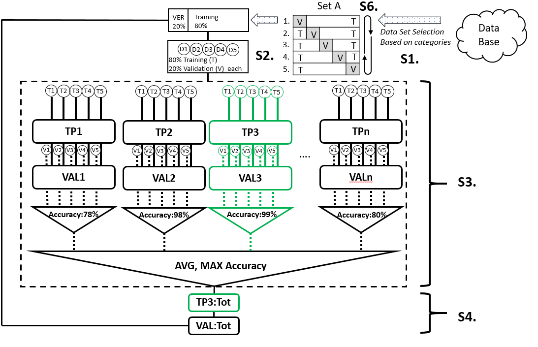
Figure 1. ML pipeline workflow: S1: Select data set A according to requirements. S2. Segment data as set A1 and further segment the training set as D1-D5. S3: Training and validation on segmented data set using TP1-TPn and identification of the best TP (highlighted in green), based on accuracy. S4: Training and validation of the whole data set using the best TP. S6. Iterate S2-4 when set A is segmented to A2-A5, known as cross validation. ST: training, V: validation, TP: training parameter, VAL: validation.

As shown in Figure 1, the ML pipeline in this project had a total of 6 steps. Each data set (e.g. set A) was selected based on some categories from the database (the outer loop) and it went through the ML pipeline via the cross-validation process (the inner loop). The cross-validation process divided each data set into 20% for validation and 80% for training. As one data set can be separated into a total of 5 distinctive validation sets, this training/validation process would be iterated five times. The advantage of cross-validation is that all data would be validated as well as participating in the training process. For each iteration, the training set would be segmented further to D1-D5, each of which contained an 80/20 training/validation ratio. The data would be learned using training parameters (TP) 1-n. In this case, it was the gamma and the cost. Both are parameters for a nonlinear support vector machine (SVM) with a Gaussian radial basis function kernel for classification problems. SVMs are used for classification and regression analysis in supervised learning models. They are normally associated with a number of algorithms. Kernel methods are named after Kernel functions, which deal with a high-dimensional, implicit featured statistical problems. After the TP with the highest accuracy was identified, the D1-D5 would be merged into the original 80% training set, trained again using the best TP and followed by an overall validation. This method can reduce the computational cost exceedingly.

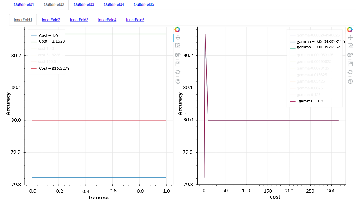
Figure 2. Prediction accuracy against gamma (left) and cost (right). The values of the gamma and the cost were picked based on experimental experience.

The effect on accuracy of gamma (left) and cost (right) had been visualised using interactive diagrams as shown in Figure 2. The outer loops were the data set selected based on the features from the database. The inner loop represents the result from each iteration in cross-validation. Normally, a high gamma leads to high-bias (high accuracy) and low-variance (high precision) models, but in this case, the gamma had no influence on the accuracy. Hence all lines overlapped each other on Figure 2 (right). On the other hand, the cost defines the soft/hard margin in the classification process. In this case, some certain cost value is better than the rest. By visualising the accuracy against training parameters, it is very easy to find the best parameters for the overall training set.

Do you get it now? 🙂

If you want to learn more about my work, please watch my presentation below: