End of SoHPC. New horizons for my CFD projects on HPC

Here we are again for the third time! Last time! What an amazing summer was! Now it is September, new projects will start as soon as possible and new adventures are waiting for me. But before going on I would like to talk in my last blog post about something useful I learned and why you should apply for this program.
Computational Fluid Dynamics Tools
In general, a fluid dynamics computation is made up of three different steps: pre-processing, simulations, post-processing.
- Pre-processing: in this part, we performed our mesh, composed of up to 46 million fo tetrahedral elements. To create the mesh, we used ANSA. Unfortunately, this is not an open-source tool, but it is available in the student version. My mate, Benet Eiximeno Franch, who has been a student during this program, provides to the team the meshes for the three different geometries.
- Simulations: this is the crucial part of the work. We selected to use OpenFOAM, which is an open-source CFD solver widely used for research activities and industry projects. We used the simpleFoam and pimpleFoam algorithm in order to evaluate the solution for the steady-state and the transient simulations, respectively. We selected to use, according to our Supervisor Ezhilmathi Krishnasamy, the RANS model based on the two equations k-Omega SST turbulence models. We also tested other turbulence models and, in the final paper, we had compared the results. What we noticed is the according to in the wake region of the k-Epsilon and the k-Omega SST. Instead, the k-Omega differed a lot from the other as a consequence that it is used to predict well the flow near the wall, while the wake region is a free zone far from the wall, indeed the k-Epsilon compute well the solution.
- Post-processing: like in all the HPC simulations, we used Paraview, which is a free open-source tool. With it, you can obtain some nice images. But pay attention! CFD is Computational Fluid Dynamics, not Color Fluid Dynamics! Each color must have a physical meaning.
Q-criterion
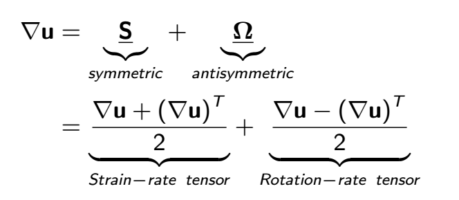
This is one of the typical visualization used to figure and draw the vortices. To understand the main idea I will explain how we computed it. Starting from the definition of the gradient of the velocity field, we can split it into two tensors: one symmetric and one antisymmetric. The first one is associated with the strain rate, while the second one is linked with the rotational capabilities of the fluid element that we are considering
From these definitions, we can build the scalar Q value as shown
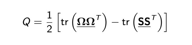
where “tr” stands for the sum of all the diagonal elements of the matrix. In this way, it is easy to understand what it shows when it is positive or negative. In particular, we have
- Q<0: areas of higher strain rate than vorticity in the flow
- Q>0: areas of higher vorticity than strain rate in the flow
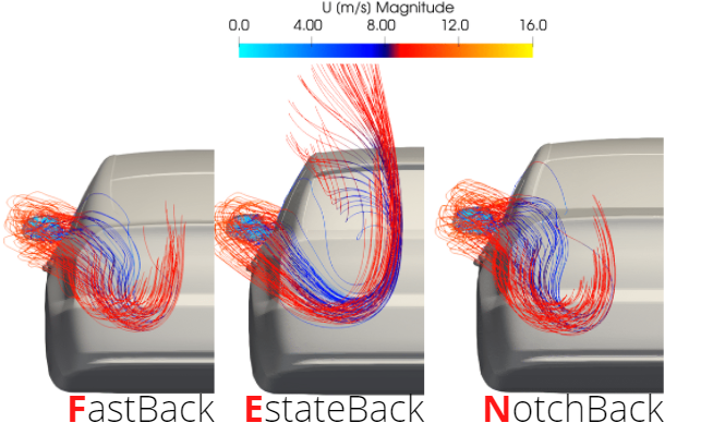
The figure below shows what is explained for Q=10 for all the three configurations: Fast-, Estate-, and Notch- -Back.

Overview of turbulence modeling
I already discussed it in my previous blog post. You can check it here.
Blunt body incompressible aerodynamics
Cars are blunt bodies. For that reason, when the Reynolds number is very high and we are considering an incompressible turbulent regime, a particular phenomenon appears. This is called the crisis of resistance, in which suddenly the CD decreases. This is also the reason why the golf balls have small pits in order to accelerate the transition of the flow from laminar to turbulent making appeared the previously mentioned effect and reducing the drag. In addition, for that reason, the CD remains almost constant with the variation of the Reynolds number. We performed several simulations for all the configurations for three different Reynolds numbers. In the picture, you can see these effects. However, if you are interested, you can ask us for the final report paper and we will send you all the details.

Rear Mirror streamlines
We analyze also the rear mirror effects on the three different geometries. You can follow the video to understand better. Anyway, I would like to give you a short introduction with the following image.
Final results
Our final results are published in our final report that you can find on the main page of the PRACE Summer of HPC programme. Here, I would like to share with you our recorded final presentation that we made on the 31st of August 2021.
Why should you join SoHPC?
Generally speaking, SoHPC is an enjoyable program. In this experience, you will learn in the first week the main concepts of High-Performance Computing with lectures hosted by one of the most important HPC research institutes around Europe. In our case, we have the pleasure to be welcomed by the ICHEC, in Ireland. We learned many important things in such a short time, as different techniques to program, python, key access.
Then, you will be divided into different teams, one for each project. You will have the pleasure of working and meeting other guys from all over Europe with passions similar to yours: HPC, coding, and, in my case, fluid dynamics. But the HPC projects that SoHPC offers are regarded in many scientific areas of interest: fluid dynamics, big data, machine learning, FEA, Earth observation, parallelization of codes, etc.
In the project you will work on, you will have the possibility to have the access to one of the HPC clusters in Europe. You can work on what you love and learn much surprising stuff. Apply and let me know!
You can contact me on LinkedIn: Paolo Scuderi. I am looking forward to talking with you!


Leave a Reply