LSTM for Time Series Prediction

What is LSTM and why did we choose to use LSTM?

LSTM, or long-short term memory, is an artificial neural network model that can process data sequences. This is especially important for time series prediction, as LSTMs can remember long term observations. But since LSTMs are powerful models, we have to be careful when using the model. The given input and hyperparameters are very important. Therefore, it is necessary not to forget the possibility of not getting proper results even though the problem is the time series.

What I want to do with LSTM?

We have a dataset of 10 nodes’ Prometheus information cleared of outliers. Using this dataset, we want to make predictions with the help of LSTM, and to find anomalies in the system with the predictions we made.

Some of the questions we will face when making predictions with LSTM will be: How much historical data will we feed and how far away do we want to predict data? Is the dataset we have enough, will it cause overfitting? What should the hidden layer size be? What should our batch size be?

Here we first decided to predict only cpu usage. Because cpu usage usually follows a trend. So if it’s high in the current step, it will likely be high in the next step. Therefore, we primarily focused on this feature only to get relatively good accuracy.

Look at the Results!

And when we started our experiments, we only used the data of one node (the node with the most job run). Since this node was in constant use, it also included unexpected spikes. So it was a node that was not easy to predict. Afterwards, we tried to obtain the next 50 predictions by feeding the last 100 observations. We fed the entire train dataset for each epoch and trained approximately 200 epochs of LSTM.

Of course, the first results we got were not quite as we wanted. But among the many parameters we can change, which one should we start with?

First of all, we stopped feeding the last 100 data, because it still showed all the information of the node in the last 50 minutes, we reduced it to 8. We also started estimating the next second CPU usage to reduce the likelihood of the model overfitting. We experimented with changing our hidden layer size from 2 to 64. We started using dataloaders. We got results by changing our batch size from 16 to 1024. Again, to prevent overfitting, we added dropouts, applied dropouts at different rates, and experimented.

In short, we did experiments using different hyperparameters hundreds of times and finally we reached some baseline results :))

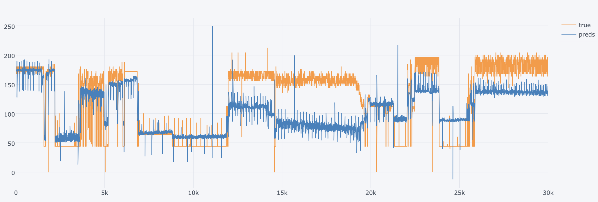
Looking at the results, we see that the model is able to predict up and down trends in CPU usage. This is good news for us! So is there still room for improvement? I wonder if we can achieve this accuracy by using less features? Is it possible to get better test loss results by changing the fed sequence length or playing with hidden size? Wait for the next post for the answers to these questions!