Revealing Mars with Programming

This blog will be mainly devoted to my project of visualizing the surface of Mars. The data used in this project derives from MARSIS radar which is carried by spacecraft Mars Express. The satellite was produced by the European Space Agency and began its journey to the Red Planet on 2 June, 2003 with the launch of a Soyuz-Fregat Rocket. The satellite consists of many components for essential working and seven instruments to study all planetary aspects of Mars. One of the instruments is called MARSIS which is a low frequency, nadir-looking pulse limited radar sounder and altimeter. It operates at the altitudes of up to 800 km above the Martian surface for subsurface sounding and up to 1200 km for ionospheric sounding. The instrument is working in 1 MHz wide frequency bands centered at 1.8 MHz, 3.0 MHz, 4.0 MHz and 5.0 MHz. It is transmitting a linear frequency modulated chirp signal with its antenna. The before mentioned antenna is a deployable dipole which consists of two 20 m elements. The peak gain of the antenna is in direction of Mars’ surface. MARSIS performed subsurface sounding in the highly eccentric orbit selected for Mars Express, which corresponds to about 26 minutes of operation. This is equal to about 100 degrees of arc on the Martian surface. Performance of the ground penetrating radar is best during the night on Mars, that is when the solar zenith angle is above 80 degrees. In this case, ionosphere plasma frequency drops significantly and lower frequency modes of operation can be used, which can penetrate deeper into the ground.

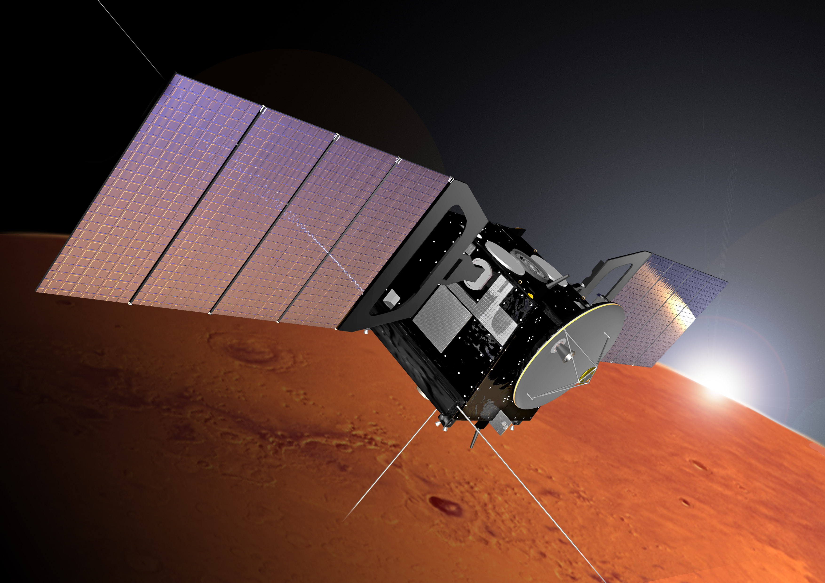
Rendered image of Marsis Express. A dipole and monopole antennas can be seen.

Each satellite orbit is well documented with 38 parameters that are kept in binary files. The data basically describes the operating mode, position, and velocity vectors of the satellite at defined position above the Mars. Additionally the most valuable data are the radargrams that contain information of echo sounding of Martian surface. They represent the strength of the received electromagnetic signal along the satellite’s path. In the database, we have 3000 satellite orbits that cover the area of south polar cap on Mars, which we are interested in. For each satellite position we can use six radar scans that differ by frequency and time shift. Each radar echo has a resolution of 512 pixels that are representing the traveling time of reflected electromagnetic signal. Traveling time is directly connected to the Martian surface and with this information we are able to reconstruct the terrain elevation. It has to be pointed out that the radargrams were already aligned with each other so the heights at the same position above the surface are the same. The alignment was done on the basis of simulation of electromagnetic waves scattering from the surface, which was scanned with a laser.

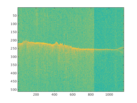
Radar echoes along the satellite path. This radargrams are used to reconstruct the Mars surface.

The next task was the construction of the functions that convert spherical coordinates of satellite movement. The planar projection was chosen which converts all coordinates into the planar Cartesian coordinate system. After that the code was implemented that automatically reads the datafiles and extracts information that we need for surface description. The routine takes into account the fact that we are only interested in the longitudes below 70°. Along with data gathering the matrix construction is performing, which effectively stores the echoes in the Cartesian coordinates. This mapping matrix had a defined resolution step and our initial resolution of topography was 2 km. Of course, higher resolution means smoother data representation but is also more computationally demanding. The mapping matrix was constructed by populating it with data from each satellite track. Because satellite orbits do not cross the south pole, we had an area there with no elevation information. An additional problem was that the satellite’s orbits are very dense around the pole and more widely spread on the borders of the matrix. This means that our data was not uniformly covering the whole area and had to be interpolated.

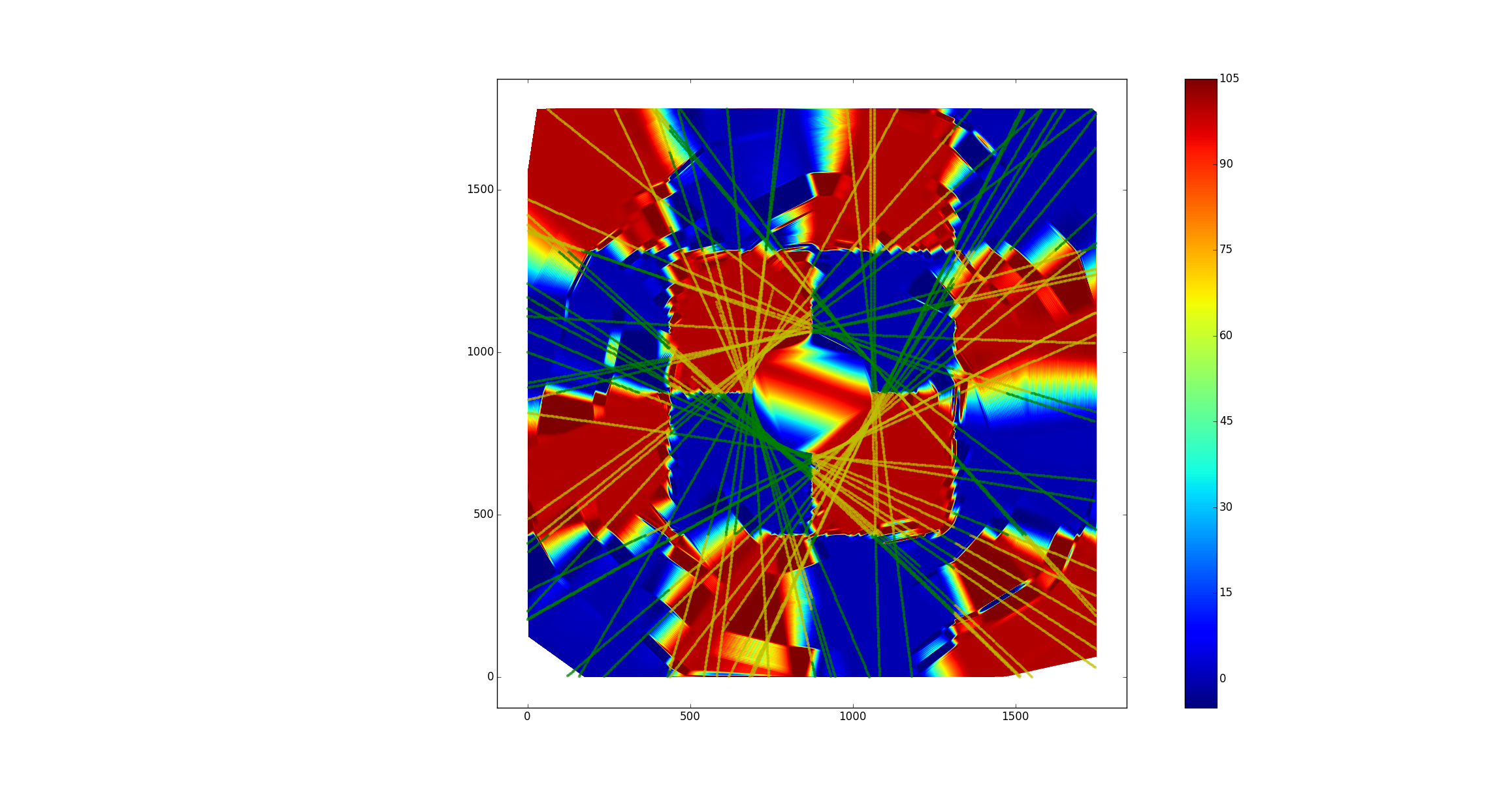
Interpolation image test with represented satellite tracks. We can see non covered area in the center.

The interpolation of the missing data is one of the most important steps in the project that is crucial for real data representation. We chose three of the most appropriate techniques that would potentially suit our needs. They are simple linear interpolation, inverse distance weighted interpolation and radial basis function interpolation. We found out that the first one was the fastest but also produced the worst results, while the last one produced the best results but was also 100 times slower due to the nature of determining weights with system of linear equations. The second one has yet to be implemented, at the time of writing. I also found out that non-uniform data input of the satellite tracks produced noise in the interpolated image that had the strongest impact on the edges of the interpolation area. The noise also lowered our resolution of terrain elevation representation, but the effect can be minimized with the higher number of orbits used in interpolation. After the interpolation the filtering takes place that uses the noise estimation function to filter out the noise in the interpolated matrix. At the moment we have some computational problems, since my session is limited to 12 hours and the computation time takes longer than that.

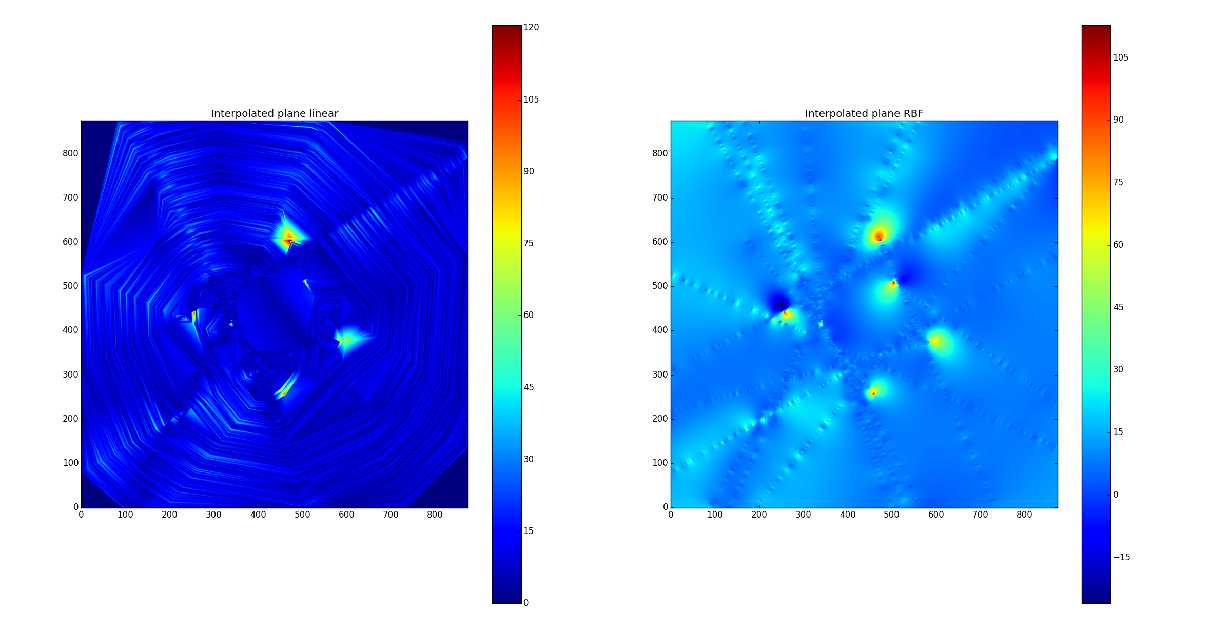
Comparison between linear interpolaton on the left and radial basis function interpolation on the right.

After we overcome the processing time problem by using bigger computer Fermi instead of Pico or by optimizing our code, we can proceed to the final step. It includes importing the interpolated and filtered matrix to Paraview, where a 3D Martian surface can be rendered and additionally modified to have accurate representation of reality. I am very much enjoying the work on my project and I am convinced that we will manage to overcome all current and future problems.

Happy programming to all of you!