The Art of Signal Processing

This blog will concentrate mainly on the processing methods that were employed for Martian surface interpolation.

Our main aim was to use single satellite tracks that provide two dimensional cross sections of the Martian surface and subsurface. Clearly, to present the surface in three dimensions we had to combine all the given satellite tracks together. Choosing the best and well performing interpolation method was not an easy task to accomplish. In the figure below we can see the result of Scipy interpolation function which is a barycentric type of interpolation. For testing purposes we used only 50 satellite tracks out of 3000 and immediately found out that the before mentioned interpolation method does not fulfill our needs. One can see in the figure below that this interpolation method does not produce a smooth surface, which is expected to be seen after the process.

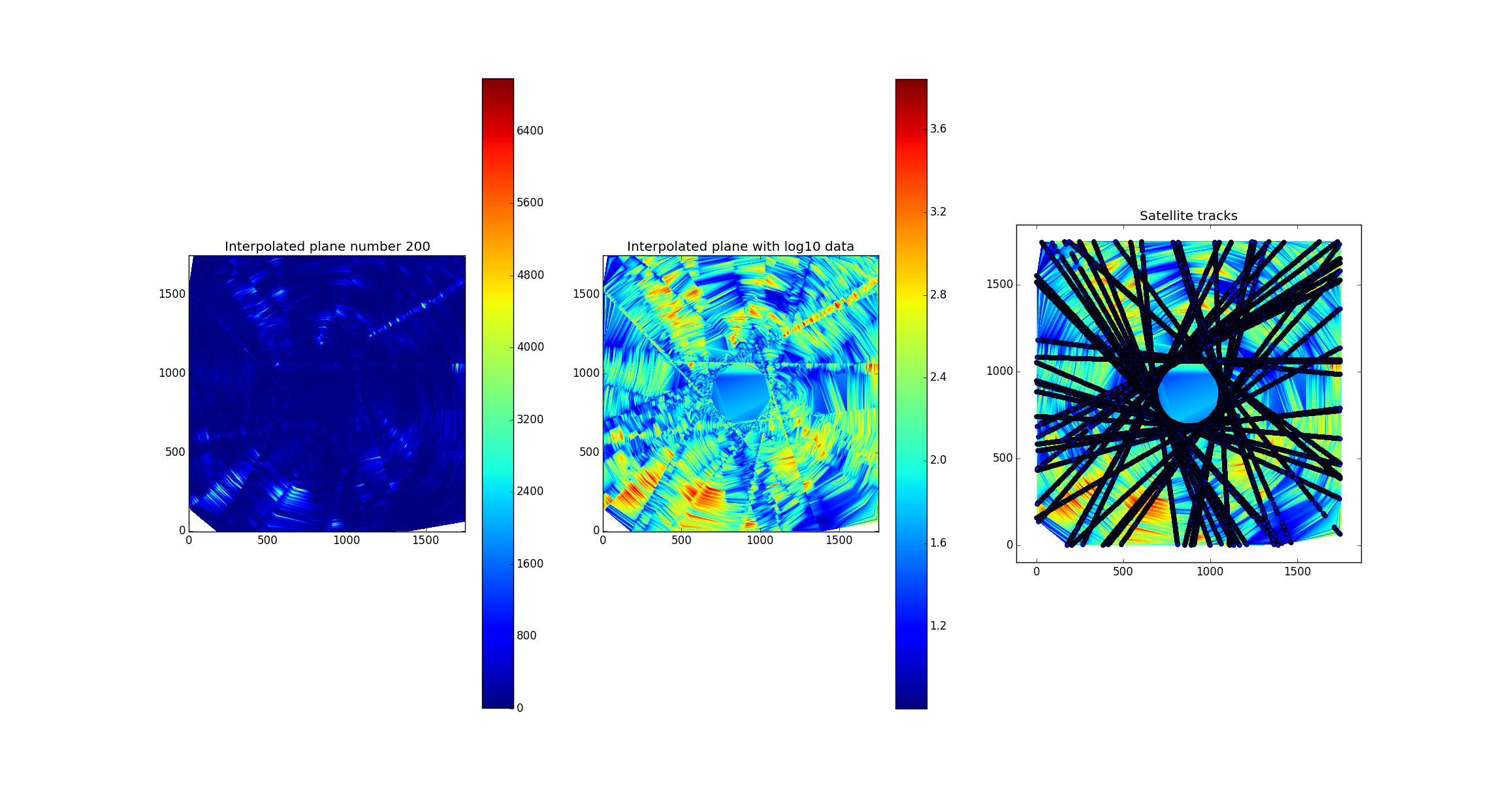
Results of barycentric interpolation. Middle picture presents logarithmic data and the right one shows the satellite tracks used in interpolation.

Since the final results were not as expected we had to find better interpolation method. Fortunately, there exists more a suitable method which is frequently used in topographical applications and is called radial basis function interpolation or RBF interpolation. Interpolated result is actually the sum of the radial basis functions that are real-valued and depend only on the distance from the origin. With the choice of appropriate function we can affect the smoothness of the end result. That is why the Gaussian function was used. During implementation of interpolating algorithm we found that the Numpy RBF interpolation function was too slow so we have decided to use the algorithm in Alglib library. The results were far better and can be seen in the figures below.

Comparison between barycentric interpolation method on the left and RBF method on the right.

Our preliminary tests were done with a limited selection of satellite tracks, so we were eager to find out how the algorithm works with all the data. Unfortunately, nothing worked the first time. In our case the interpolation process was simply too slow, since my connection to Pico computer was restricted to 12 hours. We have decided to parallelize the code and the interpolation was done in merely 40 minutes. We cut our data into the slices with the same elevation and each processor was interpolating only one elevation plane. Of course, the interpolated data was not in the final form as the original data, gathered by the satellite, was quite noisy. It is quite an art to apply numerous digital filtering and still obtain nice realistic pictures of the recorded terrain. First filter that we implemented was cancelling negative values, which resulted at some specific points during the interpolation. When all values that represented reflected power in data were positive we applied a filter for discarding data points with values below the value of average noise level. The filtering was done in the frequency domain using fast Fourier transform. The results are given below. You may be wondering what that point is in the middle. It is the Martian South pole where no satellite orbit passes and we cannot cover this area.

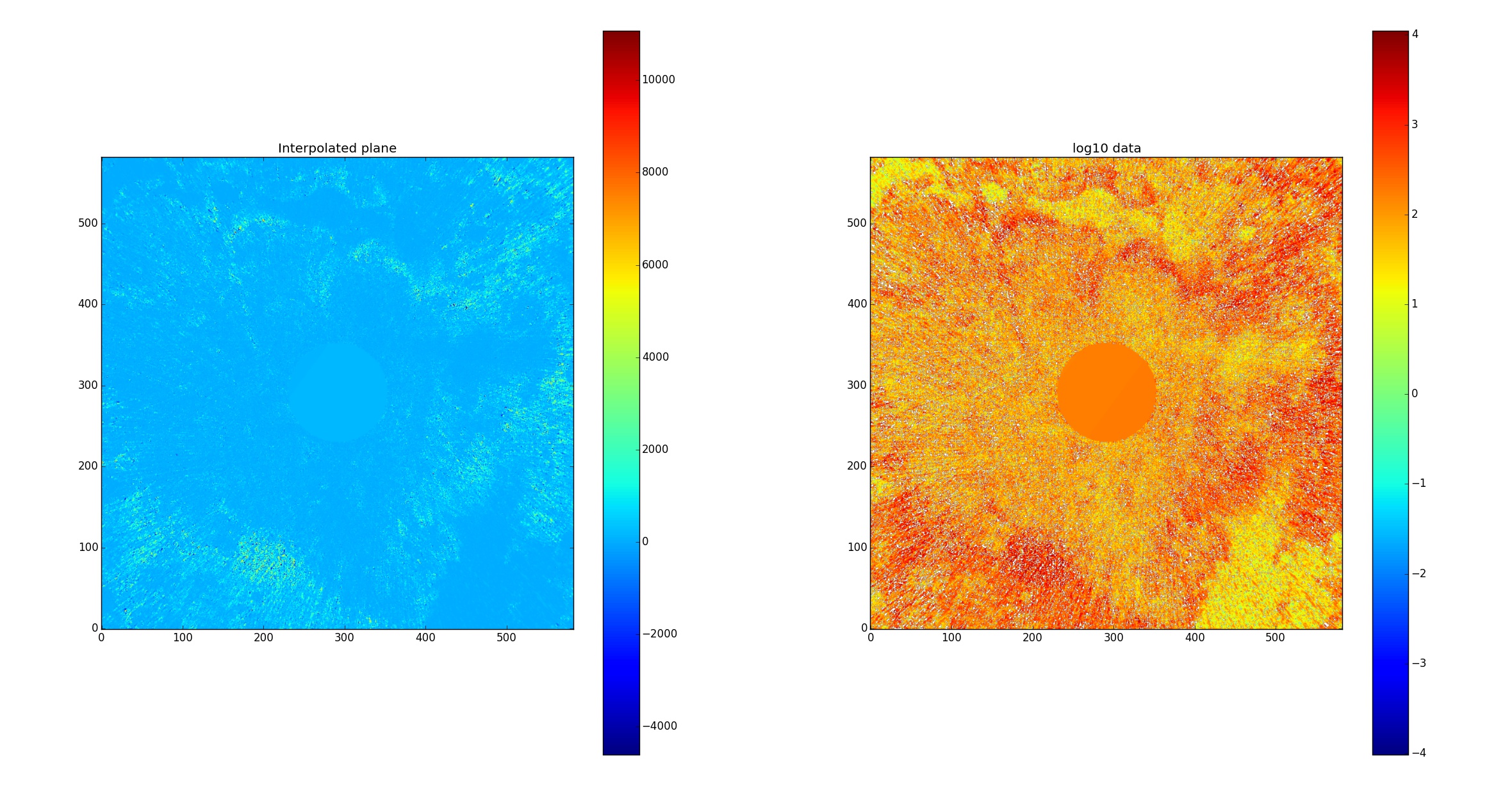
Interpolated cross section of the Martial surface on the left and logarithmic representation on the right.

At this point we could see the first nice pictures of the Martian surface but we had still some work to do. Our data points obtained from the satellite tracks were not evenly distributed and not perfectly matched along z-axis. We had to introduce further filtering in order to smooth the image and better visualize the characteristics of the terrain. We constructed three dimensional Gaussian filtering algorithm and applied it to the whole three dimensional data set. The filter had the range of 12 pixels in x and y direction and 5 pixels in z dimension. In this way we were able to produce good surface smoothing without loosing the details of the subsurface layers in z-direction. We can see the final result on the right side of the figure below.

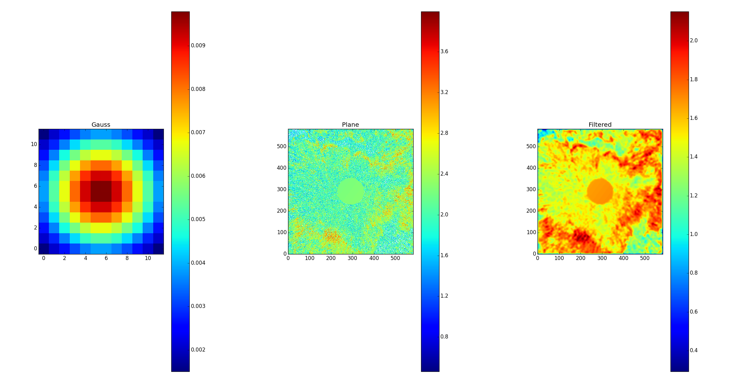
On the left is xy-plane of the Gaussian filter, in the middle is input data in xy-plane and on the right is filtered data.

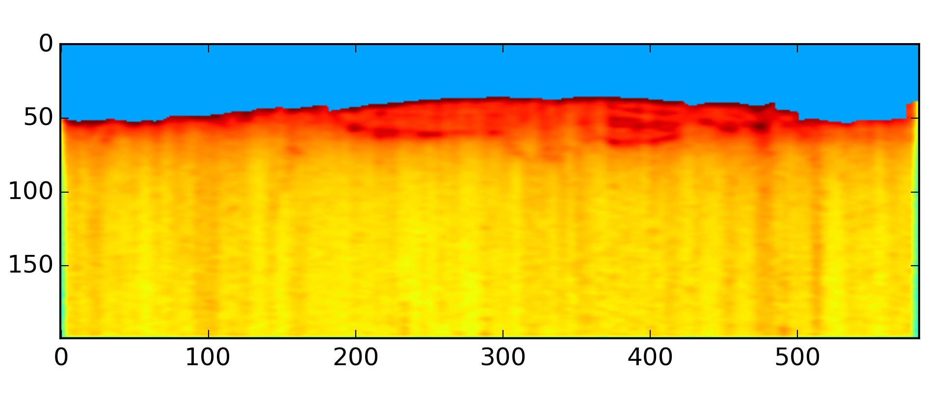
At this stage our data was finally ready to import into the Paraview and produce three dimensional renderings and visualizations. Below we can see the Martian surface along y-axis. The subsurface layers can be easily recognised and they were our main points of interest, since they can present water layers below the ice cap.

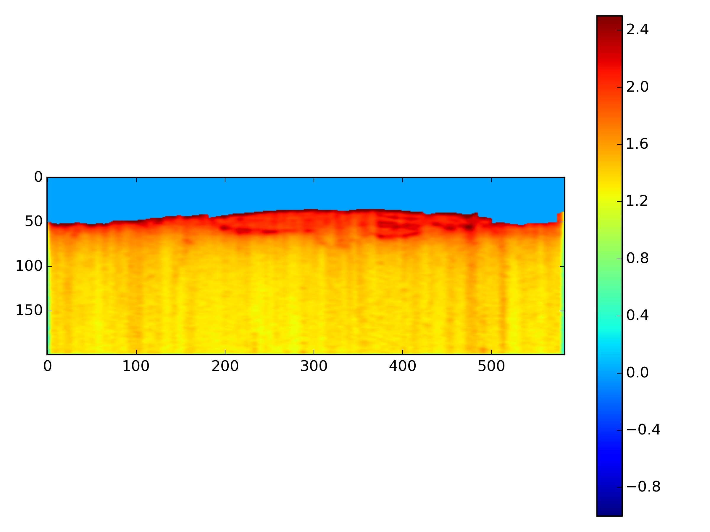
Subsurface Martian layers can be seen on this image which represent a cut 1100 km long.

We managed to overcome all the obstacles so far and the best part is yet to come. The production of the final video will certainly be a joyful experience!