Diving in the unknown: The Flow-Cutter Algorithm

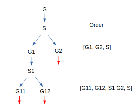
Hi ! I hope you’re ready to dive with me into this specific algorithm which will provide us a solution to our last problem. If you remember correctly, our goal is to find an order for all the nodes in a graph so that, by executing elimination, we can compute an approximation of its tree-width (max degree of nodes eliminated, we want that max as low as possible). To find this order, one well-known approach is the nested dissection. Nested dissection consists in taking a graph, computing a separator (a set of nodes), with which you cut the graph in 2 parts (or more) i.e 2 disjointed sub graphs. Repeat the same process on the 2 sub graphs until they verify some properties like “is a tree” or “is complete” where it’s easy to compute their order and tree-width. To create the final order for the root graph, start from the end by adding separators then graph orders (when they verify the previous properties and are computed directly). For instance let’s say you had a graph G, its separator is S and it splits G in G1 and G2, at this point the order is [order(G1), order(G2), S] (I write S but in reality we append all of its nodes and order doesn’t matter inside S, the only important thing is that S is after G1 and G2) . Now let us start to nest things with G1 and suppose that G2 can’t continue because it is complete. G1 will be split using S1 and its sub graphs are G11 and G12. At this point the order is the following: [order(G11),order(G12), S1,order(G2), S]. For the sake of simplicity, we will suppose that G11 and G12 are also complete to end the example here. Just one note here, our order [order(G11),order(G12), S1,order(G2), S] and this one [order(G11),order(G12),order(G2), S1 S] lead to the same tree-width so picking one or another depends on your choice when thinking about implementation. Another way to think about this approach is more visual and involve a tree like this. Therefore, the choice depends on how you want to iterate through this graph.

With that in mind we can keep going on, one question you might have is “that’s nice and all, but how do you choose your separator S at each step?” The answer is the main part of the algorithm developed by Michael Hamann and Ben Strasser in this paper. Their idea is to find a balanced a cut which splits the graph in 2 balanced parts. A cut is a set of edges (usually on directed graphs are used, so it would be arcs not edges, but in our case we consider only non directed graphs) each of those edges is a pair of nodes (u,v) so that u and v are not in 2 different sets V1 and V2 which partition all nodes V (all the vertices/nodes) = V1 U V2. To get a separator from a cut we just choose randomly 1 node per edge in the cut.

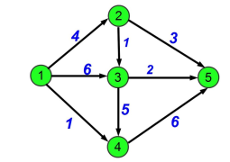
Now, onto the main part: how to select a good cut ? One specific idea in graph theory will help : the notion of flow. In some engineering problems, like computer networks, or transporting water through several pipes, you want to use the network at its maximum capacity to transport the largest amount of information or water depending on the problem. A flow is an integer value between 0 and C where C is the capacity of the pipe (i.e the maximum amount of water/info/whatever you can put in it). We also introduce 2 notions for nodes, source and target. Basically a source node is a node which creates flows so it can throw more than it receives. The opposite is the target node which absorbs flows so it can receive more than it gives. The other nodes respect the flow conservation i.e same amount of flow in and out. Here is an example of a flow graph with 1 as the source and 5 as a target, the current flow is 11 (=4 + 6 +1) and in other nodes we can see the conservation law for instance in node 2 we have 4 in and 3 + 1 out.

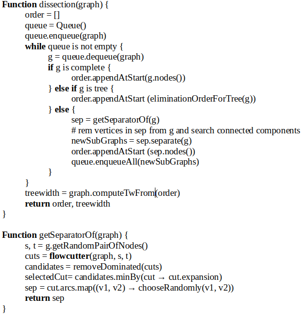
Finding the best way to flood a network to transport things from a source node to a target node is a well-known problem and it is demonstrated that finding the maximum flow is equivalent to find a minimal capacity cut. This is one of the core ideas behind the algorithm which I will explain. Another key idea is that we want a “balanced” cut which means a cut with minor difference between sizes of the 2 split vertices sets. They introduce a parameter to count this, epsilon = 2 * max(|V1|, |V2|) / n – 1 called the imbalance rate, in the core dissection part they precise to reject a cut with imbalance > 60%. To select a cut from the output cuts of the flow-cutter algorithm we will first remove the “dominated” ones i.e the ones having bigger size and bigger imbalance rate than any other one. Once we remove the worst cuts we choose the one with min expansion = size / min(|V1|, |V2|). Those wrapper algorithms can be described more easily as a pseudo code (syntax is kind of my custom fusion between Kotlin and Python) like this one :

Now it’s time to explore how the flow-cutter algorithm works and how it chooses cuts. We will use the idea of flows on undirected graphs so we double each edge to 2 arcs in both directions. All the capacities will be 1 because we don’t have capacities in the input graph we use and also because it has a clever simplification with residual graphs that we no more need to compute. The algorithm will manage 4 sets of nodes S, T, SR and TR which mean sources, target, source-reachable and target-reachable. The idea is to solve the max flow problem, find the min cut and then add source (if source reachable size is too small) or target (if target reachable size is too small) in order to enhance the cut’s balance by resolving the max flow problem and repeating the process several times to get more and more balanced cuts. The pseudo code given in the paper is the following :

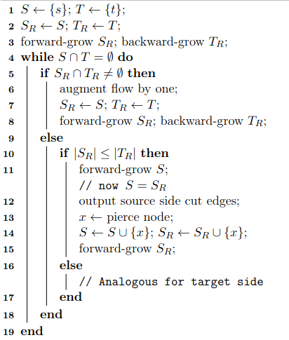
Here, the forward and backward grows are equivalents to the same process : add to the input set all the nodes such as a non-saturated path, between x in input set and y not in input set, exists. Parenthesis : forward and backward are the same because we work with undirected graphs, the difference is the direction x -> y (forward) or y -> x (backward) if you work with directed graphs. The line 12 means create cut and add it to the cuts to return at the end of the algorithm.

In a future article we will talk about complexity and performance of this algorithm on real graphs; Also will see more practical implications to enhance its result and runtime using some multi-threading.