Turbulence, Navier-Stokes equations and HPC

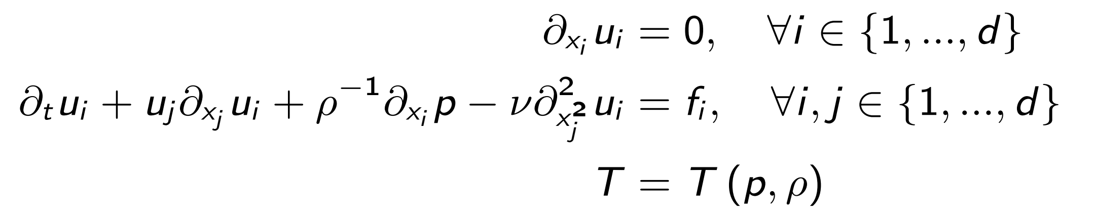
Navier-Stokes equations are a set of PDEs not analytically solved. They are one of the unsolved mathematical problems of the Millenium, which resolution will give the award from the Clay Mathematics Institute. However, they completely describe the fluid’s behavior in all situations. Navier-Stokes equations are a system of three laws of equilibrium: mass, momentum, and energy. The first one is also called the equation of continuity, the second corresponds to the First Newton’s Law, while the last one is the First principle of Thermodynamics. They can be written in different forms, referring to a finite control volume (integral form) or an infinitesimal control volume (differential form). In addition, this control volume can be considered fixed in space and time (Eulerian approach, conservative form) or moving with the fluid (Lagrangian point of view, non-conservative form).

To understand and analyze the behavior of the external or internal fluid flow, we have two different possibilities: experimental investigation or numerical approach. The first one was the most used in the first years of studies when computer architectures were not so advanced. Nowadays, with the usage of the HPC systems, the numerical approach is becoming the most important. In this context, the CFD is placed. Computational Fluid Dynamics uses numerical techniques to discretize the Navier-Stokes equations. In other words, with the CFD, we are searching for the solution at a specific point, which depends on the typical numerical method that we are using, then, we reconstruct the solution somewhere else with a technique that, again, depends on the numerical method selected. There are a lot of numerical methods: finite difference, finite elements, finite volume, spectral methods, characteristic lines, hybrid discontinuous Galerkin method, etc. All these methods use the same already explained idea. All these are already implemented in different solvers. The one that we are using is the free open-source OpenFOAM.

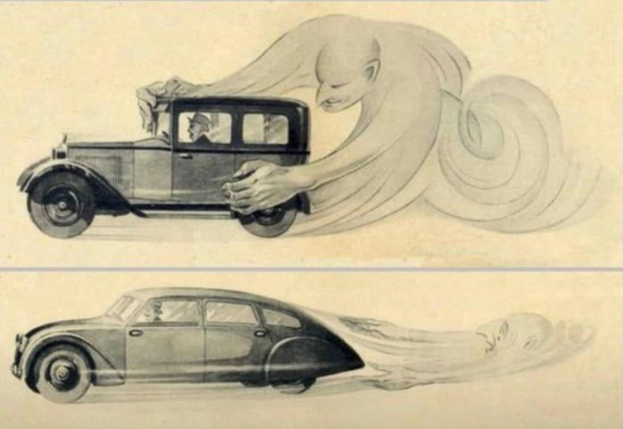
The usage of the HPC system in fluid dynamics has become interesting with the studies of turbulent flows. Turbulence is described by the Navier-Stokes equations and it is a regime of fluid motion. Even if there is not a specific definition of the turbulent regime, we can describe it as a flow with three-dimensional, unsteady, and non-linearly interacting vorticity.

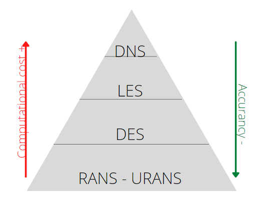
Modeling the turbulence, several methods are present in the literature. Generally speaking, the main attention must be focused on which details we want to analyze. An increment in this will introduce an increment in the computational cost. For these reasons, the DNS is not used in the industries. In general, they reach a maximum the LES, even if in the last period most of them are considering the DES. Let’s describe these from the bottom to the top:

• RANS: it is the acronym for Reynolds Average Navier-Stokes equations. With this strategy, we are decomposing the entire flow field as a sum of two different contributions: the first one is constant in time and it is associated with the mean flow. The second one, instead, is time-dependent and is associated with fluctuations. Using this decomposition for all the quantities present in the equations (velocity, density, pressure, etc.) we can see that in the momentum equation a new term appears. It is similar to stress and, for this reason, is called Reynolds’ stress. This term needs to be modeled. Hence, new equations must be added. Many numerical methods try to close the system. The classical numerical method based on one equation is the Spalart-Allmaras, while based on two equations there are the k-Epsilon, k-Omega, and k-Omega SST. URANS stands for Unsteady RANS.
• DES: it stands for Detached Eddy simulation. It is a hybrid technique that considers both the RANS and the LES approach. The idea of the DES is to reduce the computational cost of the LES but increasing the description of the RANS. It fixes a turbulent length based on the TKE and the turbulent dissipation rate. Then it compares the turbulent length with the mesh size: if the mesh size is lower than the turbulent length means that we are far from the wall, so we are interested in solving all the detached eddies, i.e. LES in applied. Instead, if the mesh size is greater than the turbulent length means that we are near the wall, thus no detached eddies are present, i.e. RANS is used.
• LES: in the Large Eddy Simulations, we are interested in solving all the large eddies, without any approximation. Then, for the subgrid contribution, we need to introduce a model. One of the most important scientists that gave a big contribution to the LES was Massimo Germano, from my home University, and Smagorinsky.
• DNS: the Direct Numerical Simulation solves all the scales, from the integral scales to the Kolmogorov scales, where the dissipation will take place. No approximation is needed, but we need to consider an increment in the computational cost. In these problems, nowadays, DNS is only used for academic works with simplified geometry, to understand the behavior of the turbulent flow under particular conditions.

In our project, we focused our attention on the RANS approach with different turbulence models: Spalart-Allmaras, k-Omega, k-Omega SST, and k-Epsilon. We use the OpenFOAM solver, which is based on finite volume discretization.

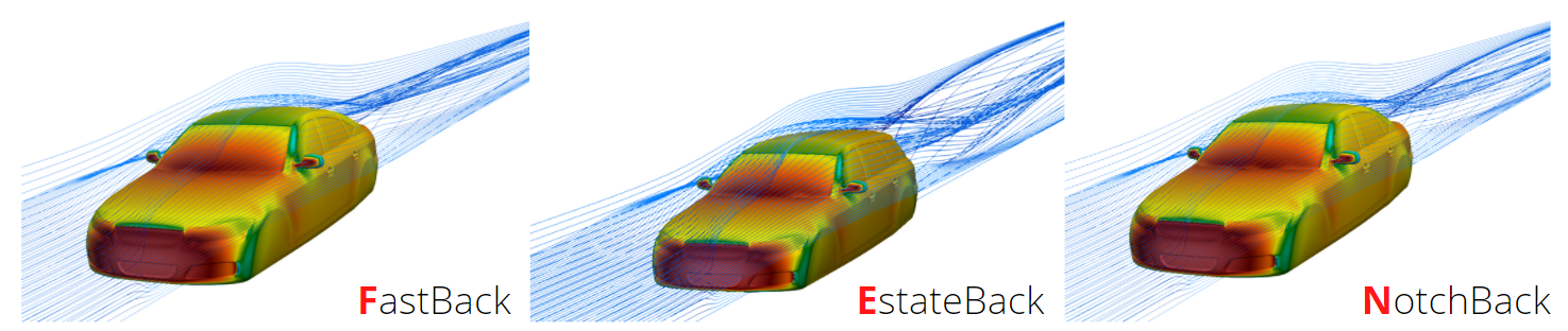
In the picture, you can see the Q-criterion applied for the three different geometries (fastback, estateback, and notchback) of the DrivAer, all without wheels following our Supervisor’s suggestion to reduce the complexity of the simulations. The simulations were running for 10 m/s inlet velocity, zero pressure gradient in the outlet region, k-Omega SST turbulence model, and for steady-states. The Q-criterion and the vorticity were computed directly on Paraview. It is simple to notice that the three different geometries provide three different turbulent structures in the wake. Obviously, big wakes mean big drag, i.e. higher request of fuel. Hence, more pollution.