If your problem is too big, make it smaller!
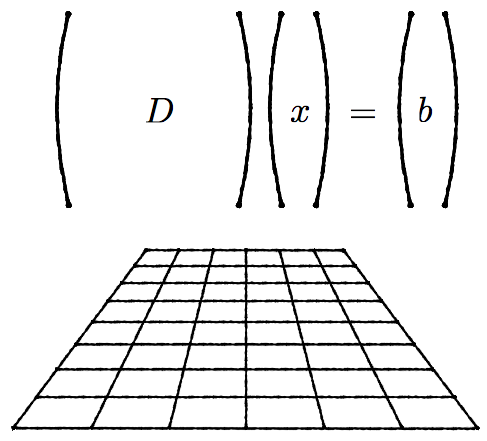
Welcome back everyone! Finally, we are ready to talk about the project. Recalling what I said in my previous post, when doing lattice QCD simulations, I said that we need to “let evolve” the quarks. More precisely, we need to compute the propagators of the quarks from one point of the grid to another. This is done by solving the following linear system:
![]()
Let’s explain what each element means: D is the Dirac matrix, which contains the information about the interaction between the quarks and the gluons; b is the source, which tells us where we put the quark at the beginning; and x is the propagator, what we want to compute.
Naively, one would have the temptation to solve this problem by just doing x=D-1 b. But if I tell you that the Dirac matrix is usually a 108 x 108 matrix with a lot of elements equal to zero (sparse matrix), computing the inverse is not an easy step (almost impossible).
There are multiple methods that can handle this type of matrices (BiCGStab, GMRES, …), but the one that we are interested in is the multigrid method.
With this method, as its name says, we create multiple grids: the original one (level 0), and then coarser copies (level 1, 2…). If we want to move between different levels, we use two operators: the prolongator (from coarse to fine) and the restrictor (from fine to coarse). For example, if we apply the restriction operator on the system, we get a smaller grid, which means that the matrix D is going to be smaller, so it will be easier to solve:

Schematic representation of the multigrid method.
After solving the reduced system, we have to project it back to its original size using the prolongator. The construction of these projectors is not trivial, so I won’t go into details, but it requires a lot of time to construct them (comparable to the time it takes to solve). So, to sum up, the steps are the following:
- Construct the projectors.
- Start with an initial guess of the solution, and do a few steps of the iterative solver on the fine grid (called pre-smoothing).
- Project this solution to a coarser grid, use it as an initial guess, and solve the coarser system (should be easy).
- Project it back to the original grid, and do some steps of the iterative solver (called post-smoothing).
To convince you that this algorithm really increases the speed of the solver, let me show you a plot comparing different methods:
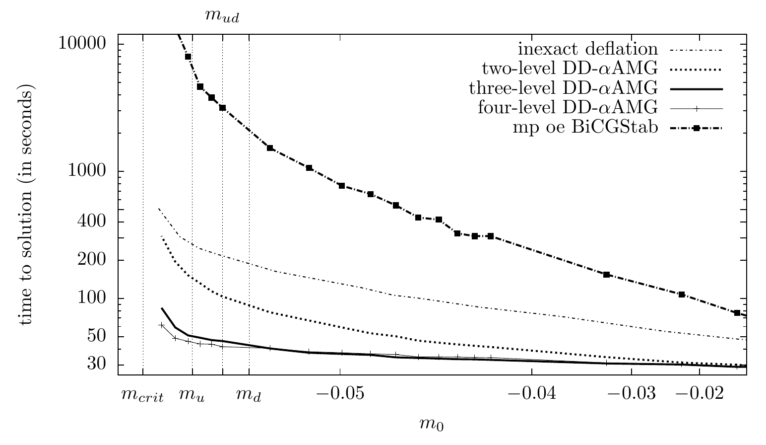
Mass scaling of diferent methods, comparing the time it takes to compute a propagator [1].
So, if the multigrid method is already fast, what can I do to make it even faster? The solution is pretty simple, and it’s the main purpose of my project: instead of solving the linear system for one b at a time, solve it for multiple b‘s at the same time. And how is it done? You’ll have to wait for the next blog post to learn about vectorization, which consists, in a nutshell, in making the CPU apply the same operation simultaneously to more than one element of an array. Cool, right?
References:
- A. Frommer, K. Kahl, S. Krieg, B. Leder and M. Rottmann. “Adaptive Aggregation Based Domain Decomposition Multigrid for the Lattice Wilson Dirac Operator“. SIAM J. Sci. Comput. 94, A1581 (2014) [arxiv:1303.1377 [hep-lat]].
