Hello, with this post I would like to give an update about my project and other interesting activities. My current progress is mainly related to exercises for using vectorization and the Xeon Phi co-processors and therefore it would better to talk about the physics involved with my project in a later blog post. Currently I am practicing on using different methods to accelerate scientific workloads on modern processors. I also compare the performance of a dummy application using different compilers and optimization techniques.

Today’s processors feature faster operations over vectors of data. They offer SIMD (Single instruction, multiple data) instructions which means you can instruct the processor to calculate multiple numbers (e.g the addition of 2 vectors of 4 double floating-point numbers) with a single assembly instruction. This is faster because usually in conventional serial programming each data operation requires a single instruction (SISD – Single instruction, single data), and therefore there are more instructions to be processed for the same amount of data.

Traditionally, computer architects have been adding smart mechanisms to the processors to increase performance, apart from improving the manufacturing process and the transistor count it allows. Such smart mechanisms include the implementation of out-of-order execution and prefetchers. Out-of-order execution tries to automatically reorder the last N number of issued instructions to avoid under-utilization of the CPU from pending memory access requests. Prefetching tries to guess and fetch the required data just before they will be accessed to hide the memory latencies. I would say the combination of the two mechanisms could compete the vectorization approach for performance increase, but it is less scalable especially when trying to increase the number of cores on a chip, due to the significant hardware complexity overhead that comes with adaptive mechanisms. It seems that lately, the processor manufacturers favour adding more vector registers and functionality to their chips and it would be very sensible if the software was designed to utilize these registers for better performance. It is important to note that SIMD instructions were already used in GPUs for many years, due to the regular access patterns of the graphics software. The real challenge is to try to exploit vectorization in scientific software either by hand or to help the compiler do it automatically.

During the last week I was also involved in other interesting activities such as a bike trip with Antti, building a time-lapse video of the Jülich sky and leaving for a weekend for my graduation in England.

My apartment is on the top floor of the highest building in the area. It also has big windows that allow me to enjoy the landscape. It also happens that I always carry with me a Raspberry Pi, which is a small Linux computer with endless capabilities. This was the perfect opportunity to program it to make a time-lapse video of a cloudy day here at Jülich. It has been capturing one photograph every 2 minutes for a day and then it has produced the video by using FFMPEG. You can see the resulting video below or a portion of it in the post thumbnail.


Visualisation is realising a growing recognition as a pivotal part of the data analysis process. As the title suggests, the project aims to avail data visualisation to help the climate research community answer or discover interesting questions about the field. The project particularly adopts interactive visualisations in order to adequately explore and communicate the understanding of large-scale climate datasets.

Data visualisation can be ideally described as the transformation of the symbolic into the geometric. Various benefits can be gained through data visualisations. The pictorial representation of data can help answer or discover further questions. The usefulness of exploratory data analysis using visual techniques was early introduced in John Tukey’s landmark textbook Exploratory Data Analysis.

However, visualisation has gained particular significance in the wake of Big Data analytics. Exploratory visualisations have become an imperative tool which allows us to discover and summarise the main characteristics of such large-scale datasets. In our case, the project deals with large-scale datasets of climate research. The data were formerly produced by climate simulation models using the WRF software.

We mainly aim to build a dashboard that can foster climate research in a twofold aspect. First, the dashboard can be used to facilitate the organisation and indexing of climate data. As climate simulation models produce huge amounts of data, it is necessary to automate the process of archiving and indexing of data and metadata as well. Second, the dashboard is intended to provide interactive data visualisations. The visualisations are intended to be produced in a web-based format, which can be interactively explored through the web browser. To achieve this, we utilise Python along with the visualisation library Bokeh. The figure below provides an overview of the project development stages.

Figure: Project Overview.

El Niño-Southern Oscillation (ENSO) is a major climate pattern that consists of oscillations of the meteorological parameters in the equatorial Pacific ocean. It happens every 2 to 7 years but it is not periodically stable.

Normal climatic conditions and El Niño conditions in the Pacific Ocean

What is ENSO?

Normal weather conditions are the following:

  • Low pressures (L) in the Pacific islands, causing rainy weather and warm ocean waters.
  • High pressures (H) near the eastern American coast, causing colder ocean waters and less rain.

When ENSO happens, this situation is drastically changed:

  • The low and high pressures switch places (this is why it is called Southern Oscillation), causing the rain to move towards the west.
  • Because of this, warm ocean waters move towards the west, causing alterations in the fishing patterns in South America.

ENSO is a phenomenon that involves the ocean, the atmosphere and the land in such a huge scale that it affects weather in the entire world, changing precipitations, temperature and wind flows along Earth. Among all of these consequences, we can highlight the following ones: massive forest fire in Indonesia, since it stops raining in that zone, flooding in Peru caused by a severe amount of rain in a small period of time, drought in India because of abnormally light monsoon months and an overall warming of the global climate temporarily.

All of these makes ENSO an important part of the weather climate cycle, a phenomenon which is worth studying and that is why I am working at the ICHEC in Dublin this summer.

What am I doing in Dublin?

First of all, I will analyze how past El Niño events have been, whether it is possible to find some trend in these events and I will also check how future El Niño events are predicted to be. Secondly, I will study how El Niño impacts other parts of the world, what is the correlation between all these events and how much was the impact in the last event. Finally, I will take a look at all the available forecast systems one season ahead, to check their accuracy and precision in detecting future El Niño events.


Abnormal ocean surface temperatures [ºC] observed in December 1997 during the last strong El Niño. Source: https://commons.wikimedia.org/wiki/File:El-nino.png

Why is it called “El Niño”?

El Niño is a phenomenon that takes places, normally, all year round but the moment in which water warms the most in the Peru coast is in December. This is why fisherman associated this phenomenon with the Christmas holidays and called it “El Niño” that literally means “The boy” after the nativity in the end of December.

Almost two weeks have passed since my first visit to EPCC at the University of Edinburgh. I met my mentor in the first week and we’ve started working on my project from the first minute of our meeting. A little background story for the idea of a project:

Online visualisation of current and historic supercomputer usage

Edinburgh Parallel Computing Centre is a supercomputing centre based at the University of Edinburgh. It houses the UK national supercomputer service called ARCHER. There are a lot of projects and communities that rely on this machine in their everyday research. It is a crucial, scientific instrument for many different people, not only academicss of the University of Edinburgh. ARCHER has an active user base of over 3000 users! It is said that a picture is worth more than a thousand words so check this infographic:

In order to build such a data visualisation page, we have to consider a number of topics. First of all, we have to get a data from EPCC servers. It’s not the same case for current and historic data. Next, data has to be preprocessed by the back-end and stored in a database that will allow fast read/write operations, periodic compression and will be able to process large datasets. Furthermore, we must look into one of the basic visualisation problems: What data should we visualise? Which part of data is the most important one?

Moreover, we have to prepare the design of this page and decide which framework we should use for the front-end development. The last one was the largest question of this past week. D3.js is the obvious choice for SVG manipulation. But this page should contain an extensible user interface that can lead to complex logic. This means that we should use one of many MVC frameworks. I’ve some experience with React, Angular and Vue. In my opinion, all of them are great, all have their good and bad design decisions. However, I find it nice that we can combine the imperative style of Angular with the declarative approach of D3. Furthermore, I hope that making an experience with Angular will be a good choice for my future self.

After an exciting training week in Ostrava, Paras and I had probably the most convenient travel possibility to our site because Leon brought us to Ljubljana by car. On the way, we made a small detour to listen to a concert of a youth orchestra where Leon’s daughter plays clarinet which was great. I was reveling in nostalgia because it reminded me of the times when I played in a youth orchestra. Also, the scenery was simply amazing with the mountain ridge in the background of the stage. Late in the evening we arrived at our destination and we moved into our beautiful dorm room in Dom Podiplomcev where we even have a balcony!

On Sunday, still tired from the training week we thought that we could finally catch up some sleep. According to the plan, our first day at our new working place would start at 9 am. That is actually late enough to sleep in. But this thought was immediately interrupted when Leon called us right before we set the alarm clock for the next day. He announced that the next day, early in the morning we would travel to the Italian border to visit the largest supercomputer of Slovenia called Arctur. The good news definitely predominated the bad news. It was very interesting to see how they set up the processors in a literally circular manner around the air cooling system. Unfortunately, we were not allowed to take pictures.

In the afternoon we were introduced to the other students and employees who work in the same laboratory. The working atmosphere is pleasant and we had lots of discussions (not only) about HPC which is nice. The job is very demanding and therefore they offer coffee for free. Since the canteen of the faculty of mechanical engineering is (for certain reasons) closed during the summer, we usually go to other canteens or student restaurants for lunch.

At the dragon bridge

Ljubljana is a very modern city which offers a great hospitality and quality of life. You can find parks everywhere and even in the city centre it is very green. In the first week, Paras and I registered for the public bike sharing system and since, every morning we go to university by bike. On the weekend, my girlfriend Alexandra visited me and so, the three of us went to Ljubljana’s castle which is a key landmark of the town. Inside the castle there’s a museum exhibition on Slovenian history.

Paras, me and Alexandra at the castle

Now, I’d like to say a few words about the project itself. My mentor Prof. Povh received a request from the area of biomedicine where they try to investigate the relation between different biological objects containing various information. One can comprehend these objects as networks. To mine (“extract”) all similarities between these networks we use the so called matrix trifactorization which can basically be reformulated as an optimization problem:

min (\sum_i R_i - G S_i G^T)
s.t. S_i \in \mathbf{R}^{k\ x\ k}, S_i = S_i^{T}

A typical approach to solve this optimization problem is to derive the Karush-Kuhn-Tucker conditions and apply iterative methods on the first order condition. Initially, we chose the fixpoint method and the projected gradient method as such iterative methods. During the first week, I have implemented the C++ code while I started using the supercomputer during the second week in order to improve the code further and to use the Intel-MKL library.

Currently, I am testing the code on real data. To show you some results, you can see a figure of convergency in the following figure. We consider RSE as a quality measure of the factorization and observe it throughout the iteration process. It is defined as:

RSE = \frac{\sum_i \vert\vert R_i - G S_i G^T\vert\vert^2}{\sum_i \vert\vert R_i\vert\vert^2}

Keep in mind, that the RSE should be decreasing and reach a small value, preferably as close to zero as possible at the end of our iteration process. But this is only possible if we choose a large enough inner dimension k < n, where n is the size of the square matrices R_i.

So, let’s take some random sparse matrices R_i \in \mathbf{R}^{10\ x\ 10} into account which we want to decompose. Suppose, k = 7. Then we achieve the following result after 1000 iterations for also randomly chosen starting point matrices G and S.
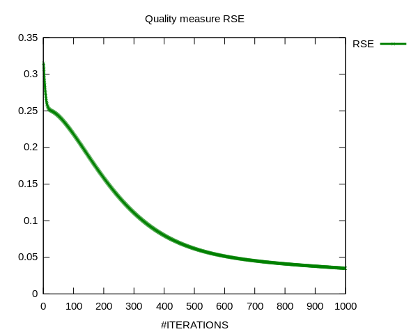
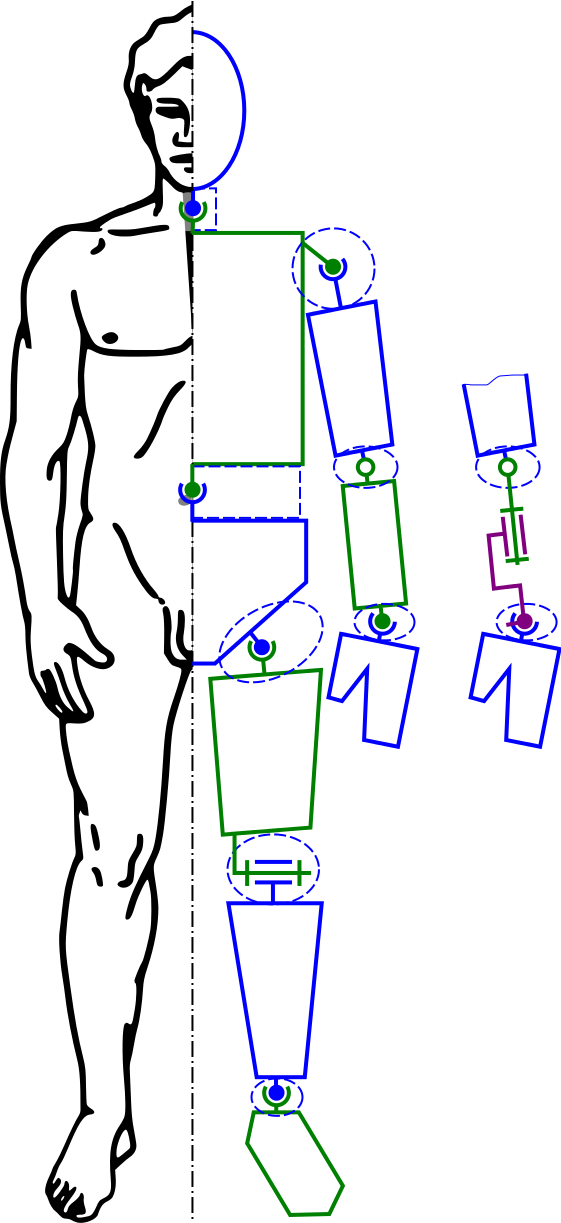
Trend of RSE for 1000 iterations


In my next blogpost, I will go into more detail about the results. Also, I will compare both the fixpoint method and the projected gradient method on real data.


Be it in films, visual arts or computer games, photorealistic rendering of a virtual scene has been a hot topic for decades. The ultimate aim of my project is to create a photorealistic render of a simple scene like the one shown above using what’s known as radiosity. Let’s dive into a brief introduction to the whole thing.

Rend ‘er? I ‘ardly Know ‘er!

So what is rendering? Well, stored in the computer is only the description of the geometry. For the box shown below, only the location of the faces are stored. Rendering is simply the process of turning that description of geometry into an actual image you can see. Boom.

The standard way to render a scene is to choose a virtual camera position, take the geometry that the virtual camera is “seeing” and draw it to the screen. For a simple box, ignoring perspective, that looks like this.

Orthographic view of box wireframe

Using perspective to make the box appear like it would in the real world look like this.

Perspective view of box wireframe

What about colour? Simply drawing solid colours looks a little strange, see?

Solid filling of faces with flat colour

What we really want is to be able to add a virtual light to the scene and give the box some kind of shading. Adding a light behind the camera produces this kind of image.

gouraud shading box graphics computers programming code

Box shaded using Gouraud shading

So What About the Rad Sounds of Radio-City?

The shading used for that last image uses a simple method called Gouraud shading. It’s straightforward and effective but all it does is calculate how much each bit of the geometry is directly affected by each light in the scene. Take a look at the room shown on the first picture, there’s only one light, a white light, and yet the box on the left is coloured a little bit red because of the red wall. Here we have a case of light bouncing off one object and affecting another and Gouraud shading doesn’t (easily) take into account. So, we turn to radiosity.

To give a quick definition, radiosity is simply a measure of how much light a little patch of a virtual scene is giving off. This amount of light produced is dependent on two things, how much light is hitting the patch and bouncing off, and how much light the patch itself is emitting. We use this to render a scene by considering how the light given off by each patch in a scene affects every other patch, taking into account how it bounces around the space. We can then properly colour a scene using the calculated radiosity.

And How Can I Tune In to The Visual Nectar That is Radio-City?

Calculating the radiosity of each patch in a scene comes in two parts. Firstly, the spatial relationship between any two patches must be found, this is called the form factor. It basically describes how much one patch can “see” another patch. If two patches are very far away from one another, the form factor between them will be very small, if they’re very close the form factor will be much bigger. If one patch can’t be seen at all from another patch, the form factor will be zero.

The second part comes here. With the form factors known, we can build a large linear system of equations in the form of a matrix equation that relates the outgoing radiosity of any one patch to the incoming radiosity from every other patch. By solving this equation we find the radiosity. Almost as simple as getting your car insurance through comparethemarket.com genericinsurance.com!

But How Can I Make My Own Radio-City?

A few different techniques and algorithms are used in the process of calculating radiosity. In order to calculate the form factors, a model-view-projection transformation must be set up, this allows the placement of a virtual camera on a patch in order to see which other patches that patch “sees”.

This transformation is used to project the geometry onto a half-cube sticking out of the patch (this is known as the hemi-cube approximation).

A z-buffer algorithm is then used to sort which patches are in front of other patches and then measure how much area the projection of each of the closest patches covers on the half-cube. This area is equivalent to the form factor.

Calculating the radiosity from the form factors can be done using numerical techniques for solving matrix equations but this requires the storage of n-squared numbers for n patches in the scene, which can end up being a massive amount of numbers, and a massive amount of memory, for complex scenes.

We can alternatively use a technique known as progressive refinement. This is where instead of finding out the radiosity of every patch at one time, the radiosity of a single patch is estimated based on approximate radiosity levels currently known in the scene and then we project that patch into the scene as if it were a kind of light. This process is repeated over the patches until the radiosity for the whole scene gets as close as we want to the true values.

And that’s all she wrote.

Dublin Though, Must Be Tough.

lol

Seriously though, this city is wonderful. The people are as Irish as I was expecting, which is brilliant. There are parks everywhere, nice coffee places around every corner, a plethora of dynamite folk and traditional music happening in at least one bar on every street and to top it all off <suckup>I’ve been working with a bunch of pretty damn great folk at ICHEC </suckup, please offer me a job>. I’ve managed to get to at least a hundred pubs, Dublin Maker (an art/design/technology fair), the National Botanics, the National Gallery, the Natural History Museum (aka the Dead Zoo), a cinema to see the new Spiderman (pretty good, I give it 3.5 out of 5 parallel processes) and even Galway for a few days (didn’t find a Galway girl…). On top of that I managed to see a high speed chase down one of the main streets of Dublin AND I got to play the fiddle of possibly the nicest guy in trad, Cormac, the fiddler from Lankum, check them out below.


Keep it reel, folks.

Jamie


How will Earth’s climate change in the next century? This is the kind of questions climate researchers ask themselves and the reason they develop global climate models. These are used to simulate conditions over long periods of time and under various scenarios, including factors such as the atmosphere, oceans and the sun. Understanding and predicting climate behavior comes at a price though – it is clearly a computationally intensive task and heavily relies on the use of supercomputing facilities. This is why climate models estimate trends rather than events and their results are less detailed in comparison to similar models used for weather forecasting. For example, a climate model can predict the average temperature over a decade but not on a specific day. Thus, climate models no longer scale as computers are getting bigger. Instead, climate research depends on extending the length of a simulation into hundreds of thousands of years, creating the need for faster computers in order to advance the field.

Coastal wave propagation Atlantic Veros ocean simulation

Simulation of waves traveling in the Atlantic

This is where my summer project in Niels Bohr Institute, University of Copenhagen comes into play. A number of ocean simulation models are implemented in the Versatile Ocean Simulation (Veros) framework. Aiming to be the Swiss Army knife of ocean modeling, it offers many numerical methods to calculate the state of the environment during each step of the simulation. It supports anything between realistic and highly idealized setups. Everything is implemented in pure Python in order to create an open-source model that makes it easy to access, contribute and use. However, choosing a dynamically typed, interpreted language over a compiled one like Fortran leads to heavy computational cost making acceleration necessary for larger models.

How can we accelerate climate models? Parallel computation saves the day and enables us to take full advantage of the underlying architecture. In particular, GPUs can dramatically boost performance because they contain thousands of smaller cores designed to process tasks in parallel. On the other hand, processors such as the Xeon Phi series combine many cores onto a single chip, delivering massive parallelism and significant speed-ups.

Niels Bohr Institute University of Copenhagen

Niels Bohr Institute, University of Copenhagen

In the case of Veros, overcoming the computational gap is mainly accomplished through the use of Bohrium, a framework that acts as a high performance alternative for the scientific computing library NumPy. Bohrium seamlessly integrates into NumPy and enables it to utilize CPU, GPU and clusters without requiring any code modifications. Bohrium takes care of all the parallelism in the background so the developer can concentrate on writing a nice, readable ocean model. Also, porting the parallel program to run on another accelerator does not require any code changes as the parallelization is abstracted by the framework.

Bohrium is extremely useful but naturally there are cases where automatic parallelization fails to significantly improve performance. My mission during the next two months is to profile and analyze the execution of the core methods and models of Veros in order to identify the most time-consuming parts of the framework. The next step is to optimize the NumPy code using Cython to add static types in order to diverge from the dynamic nature of the language and speed up execution. I also plan to take advantage of Cython’s OpenMP support to enable parallel processing via threads. Finally, the last task of the project is to port these time-intensive methods to run on accelerators including GPUs and Xeon Phis using parallel computation interfaces including PyOpenCL and possibly PyCUDA. Bohrium will detect that these segments were parallelized by the developer and will not attempt to optimize them. In this way, the power of handmade parallel code is combined with the automatic magic of Bohrium to produce truly accelerated ocean simulations.

Speaking of parallelism, while I will be making progress on the simulation forefront, I intend to explore the beautiful city of Copenhagen along with my friend Alessandro and take as much photographic evidence as possible. Stay tuned for more posts on both parts of the Summer of HPC experience!

  1. Mr. Anton Lebedev, Hybrid Monte Carlo Method for Matrix Computation on P100 GPUs, BSC, Barcelona, Spain
  2. Mr. Aleksander Wennersteen, Monte Carlo and Deep Learning Methods for Enhancing Crowd Simulation, BSC, Barcelona, Spain
  3. Mr. Adrián Rodríguez Bazaga, Apache Spark: Are Big Data tools applicable in HPC?, CC SAS, Bratislava, Slovakia
  4. Mr. Andreas Neophytou, Calculation of nanotubes by utilizing the helical symmetry properties, CC SAS, Bratislava, Slovakia
  5. Mr. Petr Stehlík, Web visualization of Energy load of an HPC system, CINECA, Casalecchio di Reno, Italy
  6. Mr. Arnau Miro Jane, Web visualization of the Mediterranean Sea, CINECA, Casalecchio di Reno, Italy
  7. Mrs. Dimitra Anevlavi, Development and validation of real-time earthquake hazard models, EPCC, Edinburgh, UK
  8. Mr. Sam Green, Interactive weather forecasting on supercomputers as a tool for education, EPCC, Edinburgh, UK
  9. Mr. Jakub Piotr Nurski, Online visualisation of current and historic supercomputer usage, EPCC, Edinburgh, UK
  10. Mrs. Edwige Pezzulli, Visualizing European Climate Change, AUTH/GRNET, Athens, Greece
  11. Mr. Mahmoud Elbattah, European climate model simulations, AUTH/GRNET, Athens, Greece
  12. Ms. Ana Maria Montero Martinez, El-Nino: It’s periodicity and impact on world weather, ICHEC, Dublin, Ireland
  13. Mr. Jamie Quinn, Radiosity in Computer Graphics, ICHEC, Dublin, Ireland
  14. Mr. David John Bourke, Visualization of real motion of human body based on motion capture technology, IT4Innovations, Ostrava, Czech Republic
  15. Ms. Shukai Wang, Performance visualization for bioinformatics pipelines, IT4Innovations, Ostrava, Czech Republic
  16. Mr. Philippos Papaphilippou, Cude colors on phine grid, JSC, Jülich, Germany
  17. Mr. Antti Oskari Mikkonen, Hip, hip, hooray! Get your 2-for-1 GPU deal now., JSC, Jülich, Germany
  18. Mr. Konstantinos Koukas, Accelerating climate kernels, UCPH, Copenhagen, Denmark
  19. Mr. Alessandro Marzo, Tracing in 4D data, UCPH, Copenhagen, Denmark
  20. Mr. Jan Packhäuser, Parallel algorithm for non-negative matrix tri-factorization, UL, Ljubljana, Slovenia
  21. Mr. Paras Kumar, CAD data extraction for CFD simulation, UL, Ljubljana, Slovenia

If you read my presentation blog post and you have come here expecting to see some nice visualizations about dying blowflies, then keep reading as I have a little surprise for you.

point tracking, optical flow, lucas kanade

Testing my tracking algorithm first in 2D

As you may already know, my project is about Tracing in 4D data. But what does that really mean? Well, it just means that I have to use math to track the position of an object in a 3D movie! The problem is that this task is very well studied and documented in 2D, but not that much in 3D. If you are interested in Computer vision or Image processing then you may already be familiar with OpenCV, a big and awesome library that comes packaged with every Computer Vision/Image Processing algorithm you may need and hope for, even for tracing objects in 2D videos… but not for tracing in 3D. So I need to make my own algorithm! Fortunately, math comes to help me, because the same algorithms that work in 2D can easily be extended to 3D, you just need to add one more dimension while the math stays the same! Now I just need to implement them in a parallel and high performance fashion!

At this point, you may already have some questions, like: “3D movie? Like Avatar?” Well, not really! 3D films in cinemas are not really 3D but they use stereoscopic photography to give an illusion of depth, while the kind of 3D movies I’m talking about keep the full information about depth representing each 3D volume through voxels (the 3D version of pixels in a 2D image)! That’s why they occupy so much disk space and why they are so computationally intensive to analyze and process! They are often used in the visualization and analysis of medical and scientific data as a result of a volumetric imaging technique (like Computed tomography (CT), Magnetic Resonance Imaging (MRI), or ultrasound). These techniques are now pretty common, for example my dentist asked me to do a 3D CT scan before removing my wisdom teeth!

But the real problem comes in research experiments. Europe has several synchrotron facilities (big X-ray machines) like ESRF, PSI, and MAX-IV. These facilities can produce enormous datasets, especially medical beam lines. They collect 3D volumes very fast to make 3D movies to study what happens over time. These volumes are typically very high resolution ( ~ 2560x2560x2560 voxels) and this means that if, for example, we collect a volume like this 15 times every second for 10 minutes, we get 9’000 volumes with a total size of more than 300 TB! That’s like 10’000 blu-ray discs!

tomography, reconstruction, foam, HPC,

Tomographic reconstruction of a system that is a constriction through which a liquid foam is flowing.

The analysis of this data typically involves tracing one or more objects, such as a heart clap or lung tissue, in 3D over time. Another example is the paper by Rajmund Mokso on which my project was born. Yes! It’s the one about the blowflies! He and some other guys developed a very fast and high resolution CT imaging technique to study their flight muscles, which swing back and forth 150 times per second! As promised, here you can find a visualization (that came attached to the paper) of the kind of data they collected. But the cool thing about the algorithm is that it doesn’t depend on the data and it could work on any dataset! Just this week I was handed a dataset where the system is a constriction through which a liquid foam is flowing.

So I need to get back to work and I will let you know how it goes in my next blog post!

After the stimulating training week at IT4Innovations, Ostrava we (me, Jan and our site supervisor Dr. Leon Kos) set forth on a long, exhausting but finally much rewarding drive towards Slovenia. Special thanks to Leon, as I got the opportunity to taste some delicious Slovenian food on my very first evening in the world’s first green country.  After catching up on some much needed sleep and a sneak peak in the beautiful city of Ljubljana over the weekend, I was all charged up to start with my project work. My HPC journey in Ljubljana stared with a visit to the Arctur supercomputer, one of the few privately owned commercial HPC service providers. Learning about another awesome supercomputer invigorated me to start on my project titled “CAD data extraction for CFD simulation“.

Jan in the Bubble 🙂 trying to play some tricks with soap bubbles

What is the project about ??

As described in my previous blog post, CAE  is a vital component of the modern day product design validation cycle. The CAE application we focus on in my project is Computational Fluid Dynamics (CFD), where one studies the flow of fluids, usually around some object – such as an airplane wing. The steps involved in the process are described in the figure below.

CAD, CAE, CFD, Python, OpenCASCADE, OpenFOAM

The CAD-CAE process chain

As described here, CAD model (geometry) is fed as input to the pre-processor where the problem is set up and transformed into an equation system which is then solved to get the results. One of the trickiest steps is the geometry cleanup which involves defeaturing (i.e. removal of small features such as holes, chamfers, fillets etc. which are not important for the CFD analysis and also make the meshing complex and difficult) and repairing of surfaces which may not have been properly imported in the pre-processor. Usually, this is somehow handled manually within the pre-processor but is cumbersome and time consuming. Thus, in order to “let the things flow” and to fast pace the entire process, we aim to develop a dedicated geometry cleanup tool based on PythonOCC which is nothing but a Python wrapper to the C++ based CAD modeling library OpenCASCADE. With the inclusion of this Geometry cleanup tool into the process chain, the entire process up to solving the equation system can be automated by writing Python scripts.

CAD ,CFD, OpenCASCADE, Pyhton

The CAD-CAE process chain with proposed modification

Since I was new to  PythonOCC, it took quite some time to figure out how actually the CAD data is represented in the program, how different parts of an assembly can be accessed, manipulated etc. Now, almost two weeks into it, I have already began with code development. Thus, you can expect some exciting results in my next blog 🙂

Exploring Ljubljana

I feel kind of lucky to have been offered my Summer of HPC project in this beautiful, green city. Last weekend, I got the opportunity to explore some parts of Ljubljana and also to visit Ljubljana Castle which apart from its great architecture also offers a great view of the city.

Ljubljana Castle

View from top of the Ljubljana Castle showing the Ljubljanica river

The Summer of HPC 2017 training week has long since passed and we have all

A carnival parade during the weekend of the Jazz and Blues festival.

started our projects in our respective countries. It has been about 2 weeks since we landed in Edinburgh and within that time I think I can safely say we have all settled in nicely here. I must say I quite like the lifestyle here, although I guess it isn’t much different to the lifestyle in Ireland (my homeland) and probably why I fit in so well here! Despite this, I’m still getting used to some of the words they use here and a few of the countryside accents.

Flower displays in Prince’s street gardens. The display on the left is a working clock.

For the few months leading up to this project I joked with friends and family about how I was going to be skipping the summer by living in Scotland for a few months. This (surprisingly) couldn’t be further from the truth! Granted, we have had a couple of days of dull rainy spells, but we have also had some great sunny days for exploring the city. Edinburgh is a great city to explore and to just go for walks in a random direction (you’ll always come across something cool). From Edinburgh castle to the gardens alongside Prince’s street to farmer’s markets selling all kinds of things and even a long beach to relax on, the city has something for everyone. Also one of the best decisions I’ve made since coming here is purchasing a bike and it is a nice way to travel to and from work. It allows you to take your mind of the day’s work and enjoy the weather (when it’s sunny) and the scenery.

A view of Edinburgh castle from a car park that hosts the farmer’s market every Saturday.

Now to the most important part of life in Edinburgh, the food. The fish and chips here are to die for, either from a restaurant or a take-away (chipper). It has always been one of my favourite meals and here is possibly the best I’ve had it (although the west of Ireland does it pretty good too). This is mainly due to the use of freshly caught local Haddock. However, this is not the only thing I’ve been eating (although I’ve had it more times than I’d like to admit) and Scotland has some other dishes to try out. The traditional breakfast here of bacon, sausage, egg, beans and black pudding is great. And when I mean breakfast, I mean the only proper meal you’ll need that day. And of course lets not forget the famous haggis, neaps and tatties which is surprisingly edible and pretty good if you ask me! I’d show you a photo of it but I was starving and ate it all instantly.

Ok I’ve talked enough about Edinburgh, now it’s time to tell you a bit about EPCC. At this stage, the three of us doing a project here in Edinburgh have met our respective mentor and have began working on various codes. EPCC has welcomed us with open arms, given us a work space and access to their coffee kitchen (which is always needed) and been of great help to settle into life here (especially Ben Morse!). My mentor, Nick, has already been a huge helping me get started in modifying the visualization end of his MONC weather model and we have already met several times to discuss ideas, problems/bugs and goals. I don’t feel like there’s much point showing off Nick’s model as it wasn’t any of my work, so stay tuned for my next blog post where I will be showing images/videos of my progress on the weather model!

# import Cup_Of_Tea as English_Tea
# import Blog_Post as Introduction

# Hello everyone :)

I am currently in Edinburgh, home of the biggest celebration of arts and culture on the planet, and of course I am referring to the famous Fringe Festival. But we have plenty of time until the festival begins and my blog starts documenting all the exciting cultural events that happen in this cool city. So it is just the right moment for me to introduce you to my internship project for PRACE’s Summer of HPC.

I have spent the past two weeks working at the the Edinburgh Parallel Computing Center on exciting topics that concern state of the art geological applications and the use of Python libraries – such as Sklearn, that support Machine-Learning and Scientific Computing. It seems that there has been a change of plan, as far as the theme of my summer project is concerned. So, instead of earthquake hazard modeling, I will be working on the development of an application that geologists will be using to discover the geological time in which sediments with similar properties were deposited over large areas of geophysical interest. These properties have been measured up to this day in well logging. But to further explore areas for oil and gas, or minerals requires many man-hours of the well log correlation.

So now, you will be wondering how my work might help geologists and engineers decide which regions are most suited for specific geo-technical exploration. A very useful tool for the experts in this area of study and analysis, would be the simultaneous and automatic well log correlation based on measurements over large areas of interest. Since methodologies that can be implemented in the well log correlation problem have been documented, it sounds reasonable to combine these scientific breakthroughs with machine-learning methods, for a more efficient overall documentation of an areas’ lithology in terms of facies classification based on limited well log measurements.

The project as presented above requires a lot of work, but I am more than content to work on the preliminary design and concept of this idea during my internship.

My main goal for this summer will be not only to work with a large amount of available measurements well logs data, but also to use existing models of well log correlation in the general concept of machine-learning applications using Python!!!

Just to give you a glimpse of the data available,  I provide you with a visualization of the most common parameters as functions of depth that characterize a well log, along with a colobar with information concerning the lithology of the well. Wouldn’t it be awesome if we trained a neural network to identify the lithology with only these 5 parameters as shown below?

Parameters as Functions of Depth[m] => Gamma Ray(GR), Induction Resistivity(ILD_log10), Photoelectric effect(PE), neutron-density porosity difference(DeltaPHI), average neutron-density porosity(PHIND)

Well-log correlation terminology in a nutshell :)

Well-logging : is the process of recording various physical, chemical, electrical, or other properties of the rock/fluid mixtures penetrated by drilling a borehole into the earths cruste. A log is a record of a voyage, similar to a ships log or a travelog.

Facies: It is the sum total characteristics of a rock including its chemical, physical, and biological features that distinguishes it from adjacent rock.


Is Scala better than C++?

Are Big Data tools applicable in HPC?

It’s been more than a week since the Summer of HPC program began, and these days have been quite interesting, getting to know members of the Computing Center of the Slovak Academy of Sciences and finding out more details about the project I will be working on. The aim of my work here, is to ascertain if it is useful to use typical Big Data tools to solve High Performance Computing problems. This will depend on the computational time required using tools such as Scala and Spark. This will be compared to ‘equivalent more traditional’ approaches such as using a distributed memory model with MPI on a distributed file system such as HDFS (Hadoop Distributed File System) or BFS (Baidu File System) and native C libraries that create an interface to encapsulate this file system functionalities. To be more precise, in order to perform fair comparisons, we’ve chosen the K-means clustering algorithm, rather than the initially proposed Hartree-Fock algorithm. This will be run on variable size datasets obtained from bioinformatics studies and we will compare the computational run time and time resilience of both approaches.


Dartboard

The dartboard: the missed throws are mine, probably breaking the typical π/4 Monte Carlo methods proportion


Of course, not everything in Bratislava is centered around work. The guys of the computing center have introduced me to ‘the game of darts’! My colleague Andreas has already played several times before, so he has some advantage. I find darts quite entertaining and useful to disconnect a little bit from the project and clear the mind. I must admit that I am a little bad at playing darts, as can be confirmed by the image on the left.


Bratislava city picture

The distance from Bratislava to other cities, indicated on the floor in the center of Bratislava

We have also had some time to visit parts of the city, and although it is small, I found it attractive to my liking, with multiple restaurants where one can taste traditional Slovak food. Up till now, the traditional dish I liked the most is the Bryndzové Halušky, which is basically potato dumplings with sheep-milk cheese. Also, since we are in summer, we have tried some good ice cream in Bratislava, and apparently we have been fortunate enough to try one of the best ice cream places in the city: KOUN. If you want to have a good ice cream in Bratislava, I recommend you this place to 101%.


To conclude, we also had the opportunity to enjoy the performance of a local music band, playing the song Angels by Robbie Williams – see my video below.

Figure 0: Me, travelling around the reserach center with my Tesla K40 GPU.

Forschungszentrum Jülich is quite an interesting place to work at. You can think of it as a town in the middle of nowhere where over the half of the population are scientists or technicians. The research center even has its own fire department and healthcare center! It is also surrounded by chain link fences with barbed wires, which are probably designed to keep the wildlife on the outside and the researchers on the inside. To get in you have to present your personal ID card and you ought to have it on your person at all times. The security of the facility appears to be quite high on the priority list. The whole place reminds me of Black Mesa Research Facility, but with less headcrabs. I’m not even sure if I was allowed to take photos, but I did anyway.

I am an alternative text! Pleased to meet you!

Figure 1: My field of view while strolling around. There are lots of these bizarre solar paneled boxes all over the facility. Nobody I have asked knew what they are. Maybe it’s some on-going experiment.

You can actually spend quite a lot of time just strolling around the research center. A couple of Master students I share the office with were kind enough to take me on a tour around the campus on a route called The Two Towers. This route visits the two largest radio towers the center has. As you might deduce from the its name, the route is almost as long as the trek from Shire to Mordor. But walking isn’t all I do! I also eat brunches, lunches and second breakfasts while drinking copious amounts of coffee. In addition, during breaks from all of that stuff, I have this pretty cool programming project I’m working on.

The project is basically about calculating gravitational or electric potentials caused by groups of discrete point masses or charges on a graphics card very quickly. These sorts of potentials are encountered for example, when simulating molecular dynamics, behaviour of plasma or formation of a solar system. You want the calculations to be very fast, because simulations usually require an immense number of time steps before they’re of any use. And lastly, we want to utilize GPUs, because nowadays they’re ubiquitous and offer the cheapest FLOPSs.

Figure 2: My field of view during a break from the strolling around. Walking’s serious business: note the legs in an optimal resting position. That white thing right there is my personal coffee kettle. That’s right, a liter of coffee, just for me!

More specifically, I convert existing CUDA code for nVidia GPUs to a more general, open-source framework called Heterogenous-Compute Interface for Portability, or HIP. With it, you only need to write source code and during compilation you decide which hardware to use. The framework is quite new and under heavy development, which becomes apparent when Googling the various error messages and noting the absence of hits from StackOverflow. In such cases, you need to do the figuring out by yourself! However unreasonable it may sound, this playing in the background has kept me sane while debugging my code.

The algorithm used for the potential computation is called the Fast Multipole Method. The large distribution of point charges (or masses) is divided into small boxes, each of which contains only several particles. The particles of a certain box and its neighbouring boxes interact classically using the usual formula for 1/r potentials and this is called the near-field. Everything further away is considered to be in the far-field. As it turns out, one can give an exact estimate of the potential outside of one particular box in the far-field with an infinite series of spherical harmonics. This we can of course approximate by selecting just a few first terms from the infinite sum. The more further away we are from the source of the potential, the more neighbouring boxes are included in the spherical harmonics series. By this one weird trick you can reduce the time complexity of this problem from quadratic to linear!

The coolest thing is that in some cases, this gives a more accurate result than the classical pointwise calculation of the potentials, by reducing the amount summations and thus diminishing the cumulative floating point addition error! No wonder the algorithm is said to be one of the most important algorithms of the last century.

Hi all,

Aleksander and his girlfriend Marta at the beach.

My girlfriend was visiting me in Barcelona, so we figured we had to go to the beach!

In my previous post I introduced myself and the SoHPC programme. Now it’s time for my project.

Why Crowd Simulation?

Throughout history, humankind has had a clear preference for grouping together in larger and larger groups. On the global scale, 54 per cent of the world’s population are living in urban areas as of 2014. In 1950, this figure was 30 per cent, and in 2050 it is projected to be 66 per cent. [1]

Planning ahead for this massive increase in urban population will be demanding, and having an accurate simulation to test your city’s new infrastructure might save lives. We can, using both modelling and real data, see how people react to various external stimuli such as a catastrophe or a change in the road.

What words are those?

Monte Carlo and Deep Learning Methods for Enhancing Crowd Simulation

Yep, that’s my project title. Loads of fancy, technical  words! All this media coverage of artificial intelligence and how it will take over the world is probably not helping with the confusion of the “man in the street”, how can a machine alone do my work?! Before I start talking about what I’m doing, I’ll try to quickly explain what Monte Carlo and Deep Learning methods are.

Monte Carlo Methods

Monte Carlo methods refer to methods of obtaining numerical results in which we randomly sample a small part of the whole space we would otherwise need to compute every point of. A good example is computing the total volume of particles in a box which could fit up to N³ particles. A normal way of computing this involves checking every single location, whereas a Monte Carlo algorithm might only check on the order of N locations, and then extrapolate the result. There are obvious limitations to this, but it works surprisingly well in the real world!

Artificial Intelligence, Machine Learning, Neural Networks,  Deep Learning, Reinforcement Learning… HELP!?!?!?

Artificial Intelligence (AI) can be defined as the study of intelligent agents; a device that perceives its environment and takes actions that maximize its chance of success at some goal. [3]

Historically, we can divide approaches to AI into groups of thinking or acting humanly or rationally. One way of determining whether a machine has reached human level intelligence is the Turing test. As laid out in Russell and Norvig, a machine needs to possess several capabilities in order to be able to pass the Turing test. Amongst those are understanding natural languages, storing information and using this information to reason, and to be able to learn and adapt to new situations.

Drawing of Neural Network. From Left to right, 3 nodes, 3 nodes, 2 nodes. All connected

An Artificial Neural Network. This specific one can for instance learn the XOR (exclusive or) operation.
By Glosser.caOwn work, BY-SA 3.0, Link

This last ability is what we often call Machine Learning (ML) – learning something without being told explicitly what to do in each case. There are many approaches to this; the one we will  talk about is Neural Networks (NN). The basic idea is to model the structure of the brain, and also mimic how we humans learn. We split the task into several smaller tasks and then combine all the small parts in the end.

As explained in the Deep Learning book [3], we try to enable the computers to learn from previous experiences and understand the world in terms of a hierarchy of concepts. Each concept is defined using those concepts further down in the hierarchy. This hierarchy of concepts model allows the computer to learn complicated concepts by building them out of simpler ones.

This hierarchical model, when laid out in graph form such as in the picture on the right, is what has inspired the name Deep Learning. Deep Learning is when there are a large number of
hidden layers.

A visualisation of a biological neural network.

A visualisation of a Biological Neural Network, on which these artificial neural networks are based.

I feel it’s worth mentioning that most of the fantastic progress seen recently is in this field of AI. And that it is doubtful that this transfers directly to so called general AI due to the very specialised training required. However, Machine Learning will change what people spend time on that is for sure. Certain tasks are very well suited for this specific approach and I suspect we will soon see it commercialised.

A last thing I should explain is the term Reinforcement Learning (RL). It’s not often mentioned in media, but it is one of the most successful approaches, albeit limited to few domains, such as games. The basic idea is that we mimic how humans and animals are trained. If the agent does something good, say, doesn’t crash, it gets a reward. If it does something bad, e.g. crashes or breaks a rule, it gets punished. There are many approaches to solve this, they all centre around giving the machine a function which assigns a predicted score for every action in a state. [4]


What am I doing?

My project is mainly algorithmic in nature. I try to come up with the underlying rules each individual in the crowd must follow. The main ones are not crashing, leaving the area and going towards any goal you’ve been given. A secondary goal is coming up with a nice visualisation. This is mostly already done, but there will likely be a large amount of work in transferring the algorithm.

Drawing of Markov Decision Process.

Illustration of a Markov Decision Process with three states (green circles) and two actions (orange circles), with two rewards (orange arrows). A POMDP is when some of this information is not given.
By waldoalvarezOwn work, CC BY-SA 4.0, Link

We will use a form of Monte Carlo method for solving  a so called partially observable Markov decision process (POMDP) which we will use for navigating people towards a goal.

For avoiding collisions, we will combine deep learning with reinforcement learning, similar to what Google-owned Deep Mind did with the  deep Q-network for playing Atari games, although our network will be much more shallow and far less complicated.

A last thing we hope to try, is using another branch of machine learning called supervised learning to instruct the agents on various aspects – such as some city paths are more likely to be taken. This can also be used to say that this road, which normally is the best option, at the time we want to simulate is in fact heavily congested and should be avoided.

The crowd simulations themselves are quite complicated creatures, so to develop the algorithms in the first instance, my primary weapon is pen and paper. After I have derived the idea, I implement it in the Python programming language, using a physics simulator called PyMunk and a game engine called PyGame. The biggest advantage of using Python is in fact Keras, a so called API for Neural Networks. It allows me to code my neural net in just a few seconds. Combined, these allow me to quickly test my ideas in practice.

PyGame screen in front showing Deep Learning controlled circle trying to navigate stationary obstacles. Terminal window in background with Neural Network code.

Status of project as I was leaving the office Friday 21st of July. The green dot is the one I’m training and the blue dots are stationary obstacles we try to navigate around. The background shows training data left and right, and in the background is an algorithm I’m trying to see if we can adopt. The algorithm was proposed in the paper Deep Successor Reinforcement Learning as implemented for a self driving truck in this Euro Truck Simulator 2 project.


[1] – UN World Urbanization Prospects 2014 https://esa.un.org/unpd/wup/Publications/Files/WUP2014-Highlights.pdf

[2] – Artificial Intelligence – A modern approach 3rd edition; Russell & Norvig, Pearson 2010.

[3] – Deep Learning Book; Goodfellow, Bengio and Courville; MIT Press 2016 http://www.deeplearningbook.org/

[4] – Reinforcement Learning: An Introduction; Sutton & Barto; Still in draft http://incompleteideas.net/sutton/book/bookdraft2017june19.pdf

The Biological Neural Network image comes from
http://legacy.iaacblog.com/maa2013-2014-advanced-architecture-concepts/files/2013/11/neuron-network12.jpg


It was a very very long trip, which began on Sunday at 2 p.m. and ended on Monday at 11 pm (with a 15-hours stopover in Milan), but finally, I landed in Athens!

“Athens, the eye of the Greece, mother of arts and eloquence”.

Since first sight from the plane, I understood this was going to be true love: a lively city, full of life and a sense of solidarity.

If I was made of Ethyl bromide C2H3Br, I would have evaporated already.

Athens welcomed me with a temperature of 40 degrees. Correction, 41, and it remained this way during the whole stay! The surrounding air reminded me of the feeling I had in Death Valley (California), when the thermometer read 120 F (almost 49 C).

After this first impact, things have been much better.

I spent the first training-week with Dimitri and Ioannis at GRNET (Greek Research & Technology Network). GRNET is located at Ambelokipi, a central district which hosts Panathinaikos’s home ground.

I familiarized myself with NetCDF (Network Common Data Form) files, which are used a lot in climate science, and learned how to access (also physically speaking – see Mahmud’s post) ARIS (Advanced Research Information System), the Greek national supercomputer system.

We also spent a great time together. Ioannis and Dimitri invited me and Mahmud to a special Greek dinner, and after a walk through ancient Greek ruins, I ate the tastiest grilled mushrooms I have ever tried. I still dream about having another piece of the organic watermelon I had there: taken directly from Dimitri’s garden!

“Salonique à tout prix!”

After this wonderful first week, I moved to Thessaloniki, to switch to the operational part of my project. It has been raining for the first few days, but now the sun is shining over the cultural pole of Greece. I’m revisiting the relevant literature on climatology, in order to understand which quantities are important to visualize from a physical point of view. I am very enthusiastic in deepening my knowledge on climate models, which help us understand how our climate system works and figure out possible future scenarios for our Earth.


In a nutshell, the objective of my project this summer is to develop a visualisation of real human skeletal motion based on motion capture. I will be working at IT4Innovations, the Czech national Supercomputing Center in Ostrava, where the Salomon cluster is based. The Salomon cluster is currently the 78th most powerful supercomputer in the world, and includes some specialised visualisation nodes which will be useful for my project.

The first step of this project will be to generate a 3-dimensional model of a human skeleton from computed tomography (CT) images. To do this, it will be necessary to segment the skeletal image data into a set of images representing individual bones. The K-Means Segmentation Algorithm is a simple, yet powerful, unsupervised machine learning algorithm that will be suitable for this segmentation.

Animation of the k-means algorithm. Source: wikimedia.org/wiki/File:Kmeans_animation.gif

The standard K-Means Segmentation Algorithm has a time complexity of O(n^2) , which means that it takes a long time to run this algorithm on a large dataset. Thankfully, this algorithm can be parallelised, and a group of researchers at IT4Inovations have implemented a parallel version of this algorithm using OpenMP. This implementation is optimised to run on the Xeon Phi co-processors that are included in several compute nodes of the Salomon cluster. In plain English, this means that this method for generating models of individual bones from the model of the skeleton requires less time to run using the supercomputer.

Kinematic chain modelling human body (Simplified). Source: wikipedia.org/wiki/Kinematic_chain#/media/File:Modele_cinematique_corps_humain.svg

Once I have generated mesh models from the image data, I will need to use the Kinect 2 to generate a 3-dimensional kinematic chain based on motion capture of a moving human. A kinematic chain is simply a set of rigid bodies, connected by fixed points and various constraints defining how the fixed bodies can move relative to the rigid bodies they connect to. These models are often used in robotics, but can also be useful in other fields including structural engineering and physiotherapy.

IT4I have developed some rather interesting plugins for Blender used for medical image processing on the Salomon cluster. In my next blogpost, I will go into more detail about image processing, the DICOM standard, and generating mesh models with Blender using the Salomon cluster.

As a guy from Central Europe, upon arriving to Bologna my first reaction wasn’t subtle: “Damn, it’s hot!”.  After two weeks of getting used to the weather, I can say that I am still boiling. I will return to temperatures once more in this post, but in completely different way.

spaghetti-bolognese

Bologna, the city of food. You can guess what the first thing we did was when we arrived at our apartment. Dropped the bags and right away went for the famous spaghetti alla bolognese. And I can tell you, they were superb! The “summer body” term has a completely different meaning for me now…

I can talk about all the amazing food, drinks, architecture and people all day long (the best thing for this is to follow me on Instagram) but let’s get to what I am actually doing this summer – apart from getting fat.

CINECA and Galileo Supercomputer

My Summer of HPC project focuses on visualizing a HPC system’s energy load at the CINECA facility. In less cryptic words, we monitor a lot of metrics regarding the whole HPC system starting from the core counters to temperatures and cooling of the whole room where the supercomputers are.

Currently, we are working on the Galileo supercomputer – which is the 281st most powerful supercomputer in the world, and we are monitoring only about an eighth of its nodes (64 of 516).

Now we get to the more technical and interesting part.

The metrics we measure are of several types, i.e. environmental metrics (mainly temperatures in different places and levels), performance metrics (such as core loads,  instructions per second) and many others. Actually, there are more than 50 metrics which are being monitored right now. All these are usually measured every 2 – 10 seconds and are sent via the MQTT protocol to a database cluster which stores it for 2 weeks. You may ask why store these for such small amount of time? The answer is simple. There is a lot of data. Each day the system produces around 60 GB of data. That is a lot of data to store and keep in the long run.

Some of the data that we are receiving in 2 seconds samples.

Now that we have all the data, what should we do with them? Visualize them of course! Here’s where I come in as the savior. I am creating a web application that takes the data and shows it in consumable format, mainly charts or as one single number. Of course, I am not showing all the gigabytes of data we have, only a very small portion of them which is usually defined by the job that runs on Galileo. This way it can show in a couple of different scenarios. A programmer is more interested in how their program performs and a system administrator cares about the temperatures and loads. This gives us an uneasy task of deciding what data should be shown.

cineca-cluster-layout

3D model of one of the cluster rooms at CINECA

All of this will eventually be displayed in a sexy interactive 3D model of the Galileo supercomputer. The good folks from CINECA already did the boring part, and the model is prepared for me to play with and still, everything will be in a browser. So once you run a job on Galileo you can actually see the physical position of the nodes on which it runs, how it behaves and how it influences, e.g., temperatures and power consumption of the nodes. Cool, huh?

In the long run, this web application can help people around HPC to realize how much energy and resources is needed to run their applications and make them focus more on the energy impact of their doings.

“It was a warm summer evening in Ancient Greece…”

says Sheldon Cooper when trying to teach some Physics to Penny. My story for the next two months, which I am going to explain in this blog, starts in a similar way…

It was a hot summer afternoon in Bologna airport. The plane had just landed and my SoHPC mate, Petr, and I were going to the apartment where we will be spending the next two months. It was tough at first, after a week of training with all the SoHPC students and 25ºC weather in Ostrava, to get used to Bologna’s 35ºC weather. Also there were just two of us, since everyone is now scattered around Europe. We had some time to enjoy the beautiful city of Bologna and start our summer diet of pasta and pizza. However, we were really looking forward to meet the people from CINECA and getting started with our projects. In conclusion, my summer story had just begun.

A typical evening at the center of Bologna.

I could write about Bologna and my stories here for the whole post, but that’s not what I want to present to you today. In this post, I want to introduce you to my SoHPC project which I will be working on during the summer. In my first self-introductory post I mentioned that I am working on the project “Web visualization of the Mediterranean sea”. But, why do we need a web visualization of the Mediterranean sea? What scientific use does it have? Well, this is what I’m going to explain in this post.

The Instituto Nazionale di Oceanografia e di Geofisica Sperimentale (OGS) is one of the parties involved in the European Copernicus Marine Environment Monitoring Services. Using their OGSTM-BFM (OGS Tracer Model – Biogeochemical Flux Model) code, they are able to perform simulations to study the major biogeochemical properties in marine ecosystems, with a special focus on the Mediterranean Sea. Generally, these simulations can be performed for:

cineca

CINECA’s supercomputer racks, photo taken during the visit to CINECA’s supercomputer facilities.

  • Short time biochemical forecasts that cover around 20 days and are run twice a week in one of CINECA’s supercomputers: Pico. Their inputs, also called “forcings”, come from other Copernicus’ partners, building a very complex network.
  • Climate studies that project up to 100 years into the future. In this case, surface satellite colour data can be assimilated with the model, both to improve the forecast skill and to produce optimal representations of the last decades biogeochemical state of the Sea.

Quite impressive, isn’t it?

So, what is my role then? Concerning numerical simulations, we can usually distinguish three main parts: pre-processing and set-up, running the model and post-processing the results. As you might have guessed, the OGSTM-BFM code generates large amounts of data. However, raw data are of little use generally. We need to post-process this data set and convert it to something that can be easily understood, for example graphs or maps. One of the problems OGS has in this subject is precisely how to optimally visualize the 3D data.

Chlorophyll concentration on the Mediterranean Sea. Post-processed in VTK using python, exported to ParaView and animated with Blender. Credits: “Generated with E.U. Copernicus Marine Service Information”

Tools such as Paraview and Blender can produce 3D visualizations and videos that can be easily understood. The philosophy behind these is: “an image is worth a hundred words”. Recently, these programs (Paraview in my case) have developed web-based viewers that can connect to and access the computers where the data set is stored. Then, 3D visualizations, maps, vertical sections or any kind of graphs that can extract information from the data set selected will appear in a browser. In a nutshell, as my SoHPC supervisor, Dr. Paolo Lazzari mentioned:

“We need an efficient way to explore the data.”

So, this is what I will be doing this summer, besides eating pizza and pasta. Stay tuned here to learn more about my project and follow my story!


Credits: “E.U. Copernicus Marine Service Information”


The forest is only 5 mins away from the hotel. Perfect to have a run in the morning before work begins

It has been one and a half weeks since the PRACE Summer of HPC program has begun. I have settled here very well, having a quick run in the forest just before breakfast, enjoying the singing of the birds, working on the top floor in the building with nice views and reading books in the evening (Since Dimitra and the SoHPC interns from last year have written great posts about IT4I and Ostrava, I’m not going to repeat the same remarkable things again, you can find all about it here).


Training week: We are all studying hard! Lecturers are from various universities and companies, sharing their first-hand experience in learning and using HPC

Because IT4 Innovations is the training site this year, I’ve got an extra full weekend to spare, unlike the others who have to travel to other HPC sites as soon as the training week has finished. After seeing off my new friends on their departures, I went to Globus (a big supermarket) with David, Alex, Antti and Phillipos. I was totally surprised that the Globus can entertain my special Chinese taste with rice and soy sauce.

I guess I’m also the first one who has met their mentor. On the first day of training, I happened to meet him at lunchtime and had a brief talk. As my mentor had to go to a conference in Italy the following week, we arranged a meeting just before his departure and summarised a to-do-list for the week. The main focus is to get me onboard with sufficient reading and tutorials on several Python Modules (Bokeh in particular), to understand the end goal of the project and to be able to reproduce the current data. People in the group are very nice and friendly.


Received a nice welcome pack from IT4I

Received a nice welcome pack from IT4I.

Generally speaking, our group is building a python module for measuring HPC performance at the moment. At the same time, we are also helping another experimental group to understand the bioactivity trends of their molecules. We’ve received information about the molecules from them and we are going to apply machine learning techniques to investigate the relationship between the molecules and their bioactivity.  Meanwhile, we also have to monitor the computing performance of all our jobs, to make sure that all nodes are working at their highest efficiency. As the only chemist in the group, I may also able to provide useful insights from a biochemistry perspective.

Follow by Email