Blog archives – Page 38 – PRACE Summer Of HPC

Has the rain stopped yet?

Posted on Wednesday, 24 August 2016 by

Tomislav Subic Posted in Blogs 2015 — No Comments ↓

Indeed, as the summer comes to an end I realize I had a lot of rain – both here in Scotland and on my computer screen. My project was to develop a weather visualisation application which will be used at outreach events, so lets take a look how that went.

During the project I have developed a application which will be used for outreach, to explain simulations, HPC and parallelism. At the beginning of the project the idea was to do just a weather visualisation demo, but after a few discussions with my mentor we realised that this has a lot of potential. So apart from the clouds and rain, I decided to expand the project and display some other interesting information about the performance and how parallelism is done. Also, the application was meant to be used just at outreach events, but with all its parts, it is perfectly suited to use as an education tool, which some people already plan on doing. It can be used in regular classes or in training courses both for young meteorologist and other scientist that want to use HPC and understand how it works.

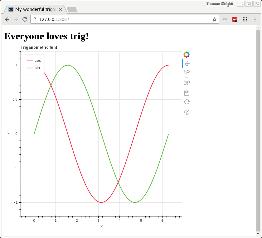
A screenshot of the application

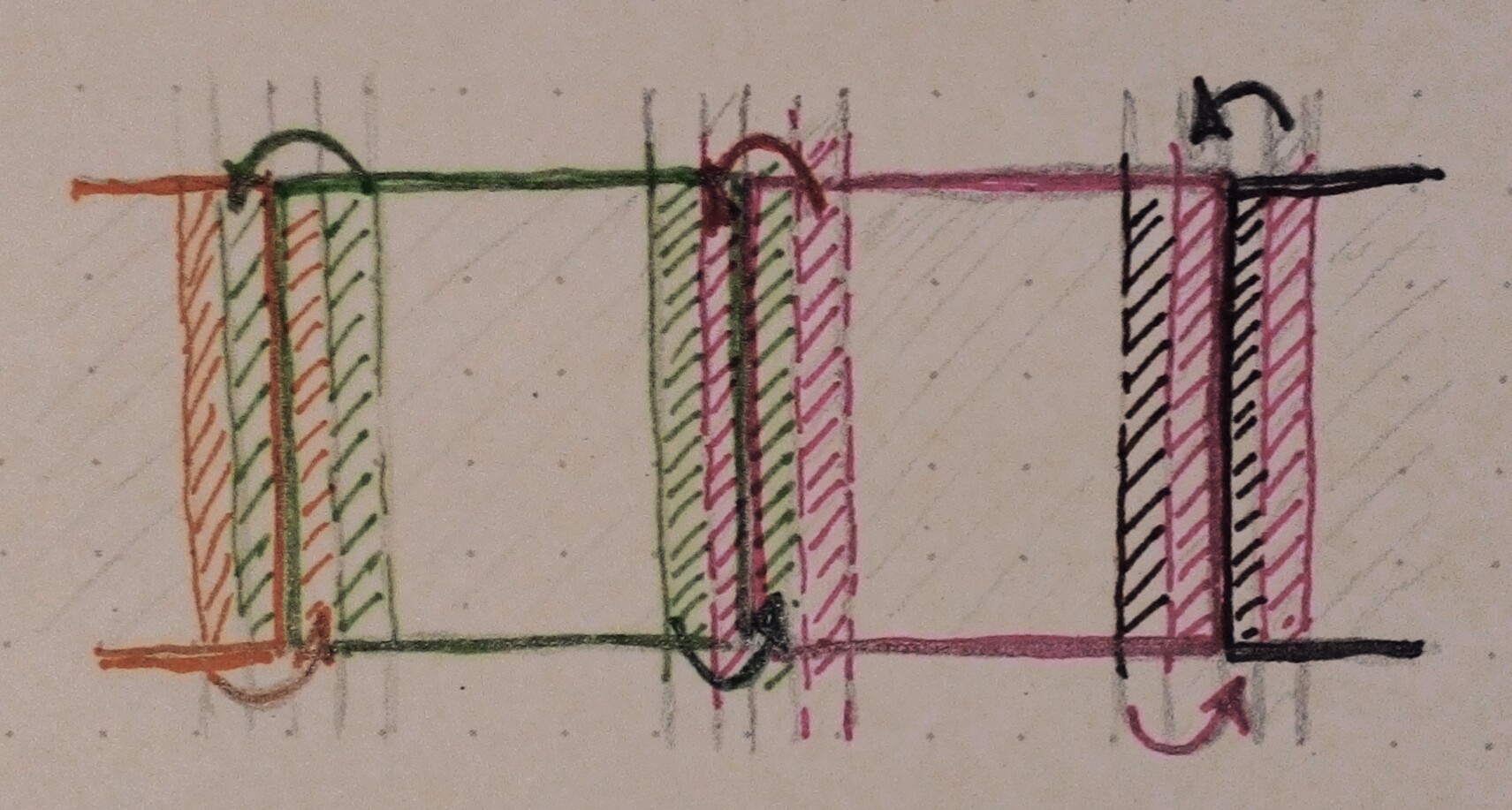
Users can select input parameters for the simulation. Of course, meteorologist use much more input parameters than the 5 we have here: wind power, atmospheric pressure, temperature, time of year and water level. They are chosen for the purposes of outreach, parameters everyone knows and can understand. Time of year translates into the force that pulls the water from the sea into the atmosphere. With water level we determine the amount of water that is available at the bottom of the atmosphere. There are some other options which do not influence the outcome of the simulation, but the performance of it. This may be of interest to computer scientist or beginners in the HPC field. Here we can select the number of cores per node the simulation will run on, but also the way the decomposition will be done. The simulation uses a 2-D decomposition technique to split up the workload amongst the nodes, although the simulated space is in 3-D. Each core will then get some piece of the atmosphere to work on, which will have a custom width and depth, but will take all of the height, ranging from the ground to the highest level of atmosphere. We set the number of processors that will split up the workload in both width and depth. We can also set one of two solver techniques: Incremental or Fast Fourier Transformation(FFT) and see how it affects performance.

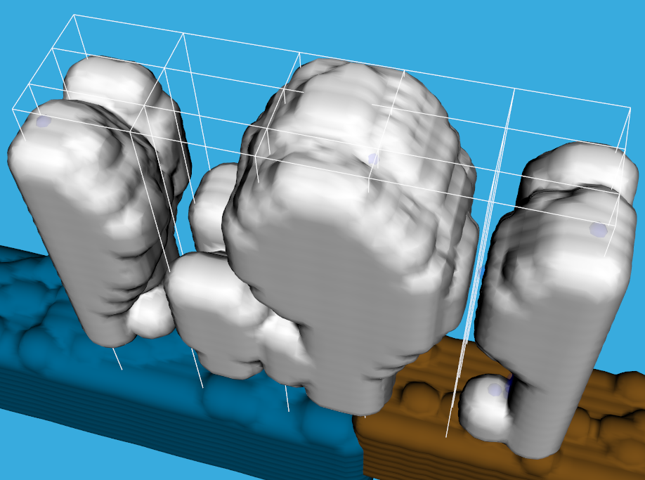
A better view of the decomposition grid

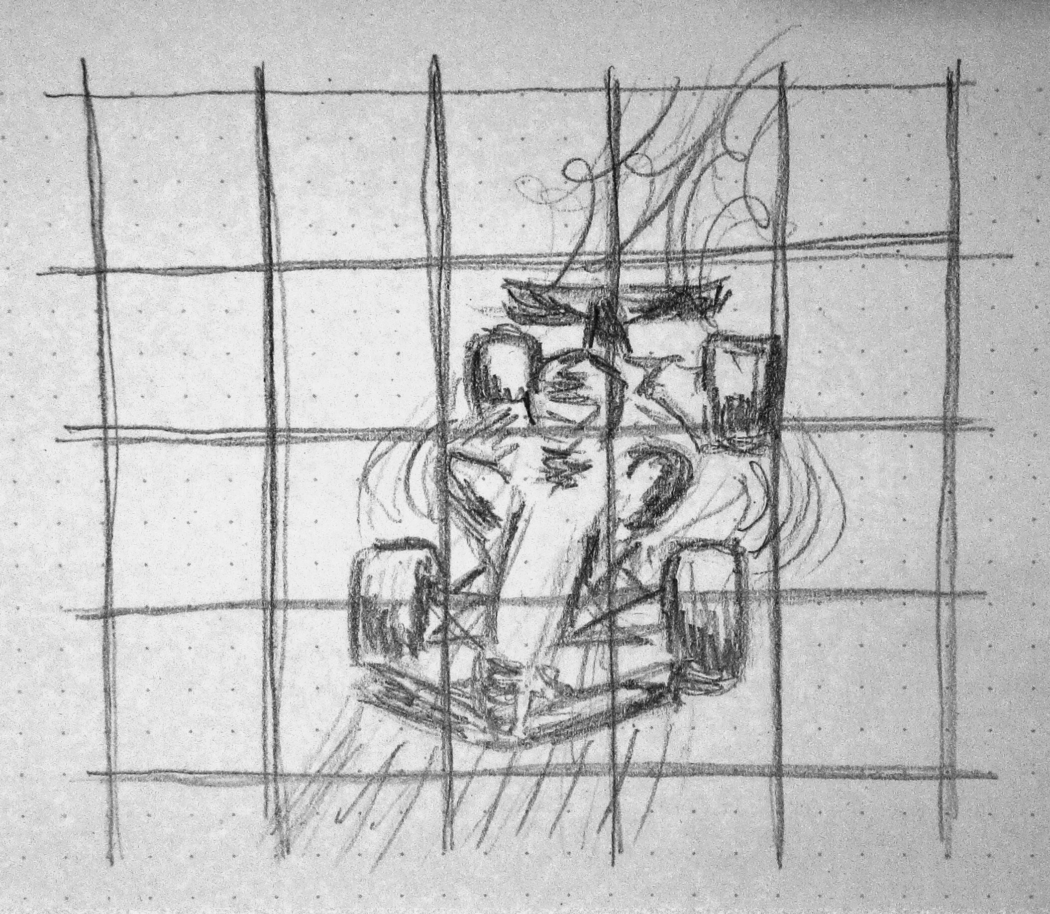
The cores in HPC systems usually have to communicate and share results and data, this communication often takes a big part out of the overall time. We agreed that it would be nice to see how different decompositions affect the communication. A visualisation is generated each time Wee Archie generates a data file. Clouds and rain are rendered, and we can see how the cloud forms and moves. If we got the input parameters right, rain will accumulate around the clouds and start falling. A gamification has also been included, if enough rain falls crops will rise out of the land, but too much rain can destroy the crops. A grid showing the decomposition is also rendered so we can see how the atmosphere is split up amongst the processes. The other part of the visualisation is the plot at the bottom part. For each core running the simulation, there are two bars; a green one showing computation time out of overall time, and a red one showing communication time out of overall time. We can then easily compare how much of the time is spent in communication and how much doing computation. Of course, it is of interest to tweak the settings so that we have low communication time and high computation time. Another performance measure appears in the upper left corner, which shows how much simulation seconds are computed in one real time second.

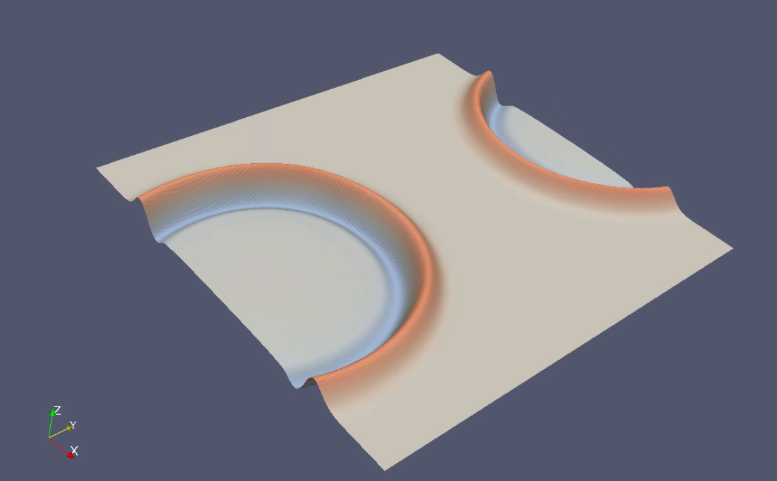
Light showers above the coast

Most scientist that are starting to use HPC are not aware of the trade-offs they have to make. Some methods in the simulations may be give the same results, but the performance is different. This application can give them an idea that performance in HPC depends on a lot of things. The decomposition grid is a perfect way to show how the data and the workload is distributed amongst the cores. With different settings and performance results we can easily show that just running simulations on a large number of cores is not enough and that we have to find the best way to distribute the workload.

The secret of Big Data programmers

Posted on Tuesday, 23 August 2016 by

Mateusz Lango Posted in Blogs 2015 — No Comments ↓

In my last blog post, I described the problem of linkage prediction in large-scale graphs. I also mentioned that this is a big data processing problem. Today I will present you one of the biggest secrets of big data programmers: the MapReduce paradigm.

First, I should mention why processing a big dataset – let say having 1 Petabyte (PB) of data – creates difficulties to modern computer systems. Well, let’s start with the most basic thing: to process the data we need to read it first. The read rate of a typical hard drive is 200 MB per second (one can argue that we can use much faster SSD discs, but they are still far too expensive to use for storage in data warehouses). So, how many megabytes are in 1 PB? It’s 1 073 741 824 MB! This means that we need 1491 hours i.e. 478 days just to read a dataset like this! And remember, the speed of writing to a disk is even lower. So how it is possible that modern big data systems need only 234 mins to sort 1PT of data (so to read, write and make some real processing with the data)? You knew it – HPC comes to the stage now 😉

If it is impossible to efficiently read such an amount of data from one disc, then you divide this data across many computers. Having 200 computers with the distributed data we are able to read this data in less than 8 minutes. That’s great, but now we have another problem: our program needs to read this data separately, communicating results between computers, and what’s more the result of our processing probably will be huge so we need to save our results also in distributed way. To make it simpler for programmers the MapReduce paradigm was proposed. I will explain this paradigm on the famous word-count example. Our task is to read a huge amount of text and return the information of how many times every single word appears in it.

MapReduce consists of three steps: Map, Shuffle (which is done automatically, we don’t need to program it) and Reduce. During a map stage, each line of the input file is transformed into one or many pairs of objects. The first object in such a pair is called “key”, and the second is called “value”. Note, that the map operation for a particular line does not depend on other lines, hence it can be executed at any time and at any node (a computer in the cluster). Returning to our example: our map will split the line into words, and then it will emit a pair (word, 1) for each word.

Exemplary execution of map stage on two nodes.

Later, during the shuffle, each node is sending all produced pairs in the map stage to other nodes. However, using HPC magic (called hash functions) all pairs with the same key are transported to the same node making further processing much simpler.

Exemplary execution of shuffle stage on two nodes.

Finally, having a node all key-value pairs related to a particular word we can reduce them into one key-value pair with the sum of values. Note that, reduce operation on a key does not depend on the other reduce operations on different keys making it possible to execute it in parallel.

Exemplary execution of reduce stage on two nodes.

And this concludes our example, because we already created the result which we wanted to get: a distributed map containing information how many times each word occurs in the file!

To sum up, MapReduce is a simple developer abstraction which allows us to write distributed & parallel applications in a simple way and it has come to be a standard in the implementation of big data processing applications. This paradigm was further extended and implemented in the Apache Spark framework (see more info in the blog post here), which was able e.g. to sort 1 PB of data obtaining earlier mentioned, awesome result: 234 minutes.

Source of featured image: http://www.thebluediamondgallery.com/tablet/b/big-data.html

Researching the center of Europe

Posted on Tuesday, 23 August 2016 by

Alejandro Rodriguez Segrelles Posted in Blogs 2015, Blogs 2016 — No Comments ↓

After the amazing training week in Juelich Supercomputing Centre where we had a brief introduction to OpenMP, MPI, ParaView, CUDA and some Team Building, it was time to start with the real business. I got into a plane headed to the heart of Europe: Czech Republic. When I arrived, my mentor came to pick me up and start this summer journey.

He showed me around. In the area there are many companies related to IT and facilities that belong to the university. I’m staying this summer in the university dormitories, just 2 minutes away by foot from the IT4I building.

The coolest building

Czech graduation tradition in the dorms

The weather wanted to stop the fun, but they were ready for it. Colours of Ostrava was the same week I arrived, and we had tickets thanks to IT4Innovations! We had our own booth where people would come to satisfy their curiosity about technology. There was some games to test people’s skills, and also one Leap device where the player had to pick up boxes in a precise way. In the spare time we were free to go to any concert, but we could listen to them loud enough from the booth anyways.

Cool guys don’t look at explosions

A wild human discovering Virtual Reality

After that, it was time to get back to work. Many hours of reading tutorials and the use of trial and error methodology were in any daily schedule. It was like being a snail, advancing slowly but surely. The main focus was to learn all I could about Unity and make a comfortable work environment.

A basic test level was made. It consisted in a demo scene with a 3D model which fills the role of an “organ” in a real level. Some functionalities were programmed at this moment as well, like making the game able to sense the mouse movement and rotate the camera or some basic controller for the player, so it could fly around the level and have the feeling it’s driving a plane. In the end, we’re going to use Spline interpolation for a predefined route in every level, but it helped me to get into the basic level of the C# API for Unity. The introduction work was done, now we will get into the real deal: medical data and actually making a game.

In the spare days, it was mandatory to explore the surroundings.

Lucky me for the second time, there was a motorbike race in a village near Ostrava called Radvanice, where they adapted the streets into an urban circuit. It was slightly bigger than just a local tournament, since there were drivers from the countries near Czech Republic.

VROOM VROOM

Despite Ostrava being famous for its excessive industries and not having that much historical places, it still has some good views and feels very cozy.

The view from the top of Nová Radnice

In the following weeks there’s more trips planned and more work to come, mainly in Blender. But for now, that’s all folks

What’s in a virtual screening dataset?

Posted on Monday, 22 August 2016 by

Juan Eiros Zamora Posted in Blogs 2015 — 5 Comments ↓

In my previous blogpost, I explained the main objectives of my project. During these weeks, I have focused towards the data analysis side of HPC rather than working on optimizing a program that runs on a super computer. I have been working to add the re-ranking functionality to ChemBioServer, which uses R scripts as a back-end to do some basic filtering on docking results. As it turns out, I haven’t actually had to interact with any of the preexisting codebase for the server – so I chose the reptile in the on-going R vs. Python war. In case you’re out of the loop, Python is a really sweet programming language for a scientist like me who is just starting to walk his first steps in serious software development: it’s fast to prototype and test new ideas on, and has a very rich ecosystem for all things data science.

In order to start getting my hands dirty, I was given a dataset of binding affinities of around 25k different compounds to 7 kinase structures: 2 ALK5 crystals, 3 ALK2 crystals, 1 P38 crystal and 1 ALK1 crystal. If this sounds like mumbo jumbo to you, don’t worry: it just means that for some of the kinases we have more than one experimental structure available, so we can make use of it as we would like our drug to bind with a strong affinity to our protein regardless of its shape, in general terms.

Where did the H atoms go? Protons readily relocate in some organic compounds, giving the ilusion that the two molecules shown here are different.

Look at the H atoms go! Protons readily relocate in some organic compounds, giving the illusion that the two molecules shown here are different. This is the most typical case of tautomerization.

The first problem I faced when analyzing these results is one which is all too common for chemists: the nomenclature of organic compounds follows a certain set of rules (that’s right, it’s got 1300 pages) that explains what the molecule is like, but still it can hide a lot of information about it from us. As a side note, I will say that this nomenclature can be absolutely hideous when molecules are big, and you don’t often hear things like this on chemistry laboratories: “Hey Johnny, do you still have some of that (2α,4α,5β,7β,10β,13α)-4,10-Bis(acetyloxy)-13-{[(2R,3S)-3-(benzoylamino)-2-hydroxy-3-phenylpropanoyl]oxy}-1,7-dihydroxy-9-oxo-5,20-epoxytax-11-en-2-yl benzoate we synthesized last week? “, so I kind of dispute it’s utility on everyday life situations (yes, nomenclature exams leave a scar on the minds of many chemists and I’m still sore about it three years after). But I’m digressing. The issue is that the classical two-dimensional drawings of molecules that you might be familiar with are a simplification of their reality. In a docking dataset, there might be several repeated entries of the same molecule. Or is it really? See, the thing is that a given molecule can have multiple stereoisomers or tautomerization states, which we want to account for during our docking calculations. So they have to be added in as separate entities even when they are not. The good news is that I’m not the first one to have come across these issues, and there now is a widely used notation to accurately describe the state of a molecule with an ASCII string. So after having parsed all the entries of the docking dataset to their ASCII representation, many of these ‘repeated’ entries in the dataset were gone.

Finally, I’ll give an overview of how the ALK2 dataset looks like by loading the results, cleaning the data and visualizing it using the wonderful Pandas library. The image below is a square symmetric representation of the binding affinities of ~25k molecules for the three ALK2 structures. We can quickly see that there is a normal distribution of the compounds for each structure, and that the 3H9R crystal has higher affinities for the compounds in general. But what is interesting is that there’s a degree of correlation which we would expect: compounds that bind tightly to ALK2 generally do so regardless of the crystal. You’ll get a better intuition of this using this interactive 3D representation. The blue line on each scatter graph is a simple linear model built by randomly splitting the data into train and test datasets, and hence you can see a small difference in the reported Variance Score for the 3Q4U-3H9R scatter plots. Now that we have a sense for what these docking results look like, we’ll explore in the next blog post how the re-ranking algorithm has played out.

Overview of a virtual screening experiment of ~25000 compounds on three crystals of the ALK2 kinase. Some degree of correlation is observed.

Overview of a virtual screening experiment of ~25000 compounds on three crystals of the ALK2 kinase. The 4 digits preceding the -ALK2 are the corresponding PDB entries of each crystal. Click here to interactively explore this dataset.

Shallow waters – the waves start to spread

Posted on Monday, 22 August 2016 by

Jiří Blahoš Posted in Blogs 2015 — No Comments ↓

The Great South Wall, Dublin Bay

I started the work on my project by exploring the provided simulation code. This is always a great adventure by its own, studying a code someone else has written before you. To those who never tried it, you definitely should. I must give all the credit to the creator of the original code, for making it nice and tidy, well structured and filled with meaningful comments. The latest one especially made my job significantly easier, and should be awarded by some sort of medal, because comments in code is something you don’t see too often, at least from what I’ve experienced. Thing that was making my progress a bit slower was the programming language used for the code – Fortran. For me, who spent most of the time coding in C++ language, the Fortran syntax was quite confusing and unnecessarily complicated at some points. But I managed to handle this little complication, and learned a new language, which is always a good thing. Also, after some initial struggles, I must also recognise some positives of the language, like an easy array multiplication syntax, without need for any library.

The next step in my work was to paralli, palare, para … Alright, the next step was to learn how to pronounce the word parallelisation properly, and also spell it right. This took me around a week, and yet it’s still not perfect, so I would like to challenge language institutes across the world to come up with a better word for this phenomena.

Anyway, the next step was to make the code parallel. I used the OpenMP library for this. The library provides a simple framework for letting the code run on multiple cores on one computational node. With my supervisor, we decided to use OpenMP for its simplicity, and also for the fact that the parallelisation (uf …) of the code is only possible over the space domain, and not the time domain. In other words, all threads must synchronise (wait for each other) after each time step of the simulation. Since the space domain is not too big in this case, one processor, equipped with 24 cores is good enough. In simple words, using too many workers for a small job can turn out contra productive.

Simulation benchmarking – each curve represents a domain of different size

Once I modified the code using OpenMP library, I was ready for some benchmarking on Fionn. I was provided with an account on this system, so I could run the simulation code on one of the Fionn’s nodes. As stated before, those nodes consist of 24 processing cores. You can see some results of the benchmarking in the attached chart. Naturally, more cores make the code run faster. Using a bigger domain results in higher speed-up, since there is less time (proportionally) spent on the thread synchronisation after an each time step, and more time on an actual work. In general, it’s clear the speed-up is not that big, considering we got only around 5 times faster run time while using 24 cores. This is probably due to the computational domain still not being large enough, and also the parallel implementation might not be the best possible one.

After debugging the parallel version of my code, and benchmarking it on Fionn, I moved to the visualisation part of my project. I started with ParaView, a software frequently used to visualise scientific data. This first required to output the data in some ParaView compatible format. While ParaView supports plenty of different file formats, it can not read the Fortran binary format. First I used the csv format. Csv is nice, tidy, simple, understandable, readable, and works pretty much everywhere. The problem is, it’s also catastrophically slow, to both write and read. So, I moved to the netcdf format, which is a scientific data dedicated file format. It’s way faster to write, and ParaView is able to read it. With the suitable file format prepared, I could start playing around with visualisation methods, displaying height maps, velocity vector fields and 3D surfaces of the shallow water simulation. At the nearby picture, you can see a sample visualisation generated from the simulation output, using 201×201 points grid, with reentrant boundary conditions (i.e. what goes out on one side, comes back on the opposite side). I am still working on the visualisation part, so I will have more material to show at the end of the project.

Shallow water simulation – 3D surface plot of the initial state – a Gaussian bump

Shallow water simulation – 3D surface plot state after a several thousands of simulation steps

During my free time, I explored a few places around Dublin. It is a very unique place. The place I live at is very close to the night life centre of the city. You basically pass one pub after another, all of them stuffed with people, with even more standing around outside of the pub. During the weekend, those places don’t sleep all night. On the other hand, you can find a large parks full of green, flowers and little lakes, where everyone can get their peaceful relaxing time. Naturally, there are also historical places to see in Dublin.

The Wellington Monument

A night in Dublin – a colourful reflections of street lights in the Liffey river

I visited the Wellington Monument, named after the British army field marshal, who defeated Napoleon in 1815 century at Waterloo. Then I went to see a place which has a big importance in the mathematics world – the Broom Bridge. It is the place where, in 1843, mathematician Sir William Rowan Hamilton wrote down his rules for quaternions for the first time.

Tne Broom Bridge

The plaque reminding Sir William Rowan Hamilton, and his set of basic rules for quaternions

Why is high performance computing so good for image analysis?

Posted on Friday, 19 August 2016 by

Marco Forte Posted in Blogs 2015 — No Comments ↓

My Summer of HPC project was officially titled “Development of a sample application in PyCOMPSs”. As you can probably tell it’s a pretty vague title, and I was given a lot of freedom to come up with my own project, which I’ll discuss a bit at the end, and also explain what PyCOMPSs is.

The general theme of my project is high performance computing applied to image processing.

High performance computing, HPC, refers generally to a computing practice that aims to efficiently and quickly solve complex problems. The main tenet of HPC I am focusing on is Parallel Computing. This is where multiple computer processing units are used simultaneously to perform a computation or solve a task. Most applications are written so called “sequentially”, this is where the computations of the program happen one after the other. There are some tasks however where the order of computation may not matter, for example if you wanted to sum up the elements of two separate lists. It doesn’t matter which you sum up first. If you could theoretically do both the summations simultaneously then you’d theoretically get a two times speed up of your application. This is the idea behind parallel computing. Supercomputers and computer graphics cards have thousands of computing units which allows them to run highly parallelized code. The Barcelona Super Computing Center has it’s own super computer called MareNostrum, it has almost 50’000 multicore Cpu’s!

MareNostrum, located inside an old chapel. Probably the most gorgeous supercomputer in the world! Image Courtesy – PRACE

Image processing and Image analysis are about the extraction of meaningful information from images. Images on computers are represented by a matrix of so called pixels, the width*height of this matrix is the resolution. These pixels contain information about the amount of red, green and blue in the image at that point. Image processing and analysis is actually a task highly suited to High performance computing and parallel processing.

I’ll give some examples, when processing an image you might only want to consider a subset of the image, let’s say you are searching for a face in the image. The face will only take up a small subset of the image so to detect it you need to be focused on that subset, or image window. Sequentially you could iterate over the image and process each subset at a time, but you could also use parallel computing to process each subset simultaneously and get big speedups linear to the number of subsets. This approach is known as the sliding window technique. More to be found at this excellent blog post, http://www.pyimagesearch.com/2015/03/23/sliding-windows-for-object-detection-with-python-and-opencv/

Sliding window example, from blog post linked.

The face might not always appear as the same size in the image however, to find it you can process the image at different scales. With parallel computing you can process the image at different scales in parallel, then process the windows also in parallel. For each image scale you take the window with the highest probability of a face detection, then you take the window with the max probability over all the scales. This is called using an image pyramid.

Image pyramid from blog post linked

For many machine learning applications, thousands of images are processed, each image can be processed in parallel also.

My project is a combination of all mentioned above. First I’ll mention the inspiration for my project. The fantastically titled paper “What makes paris look like paris?” by Dr. Carl Doersch, found here http://graphics.cs.cmu.edu/projects/whatMakesParis/ . This paper uses image processing and parallel computing to process thousands of randomly chosen images from Google StreetView in Paris and other cities to automatically extract visually coherent and distinctive images of paris, like parisian style balconies, windows and and street signs.

My goal is to develop a similar system in Python for high performance computing, but applying the techniques to images of castles in order to extract the uniquely castle like features like arrow slits, battlements, big gates and towers.

Matches from my castle features detector. Work in progress…

The PyCOMPSs system I will be using is a programming model which aims to ease the development of applications for distributed infrastructures, such as Clusters, Grids and Clouds. I will be deploying my application on the Mare Nostrum super computer.

More posts on my trials and tribulations to come!

Also a sneaky bonus pic of the excellent hiking I did in the Pyrenees.

Pyrenees hiking on Pedraforca mountain

This is happening!

Posted on Friday, 19 August 2016 by

Samanta Makurat Posted in Blogs 2015 — No Comments ↓

According to a plan, last week I’ve finally started my first proper simulation. That means, that upcoming one will finally be more chilled (hopefully). I transferred the files from Maestro to Gromacs, solvated, added ions, minimized, equilibrated (see tutorial, but don’t think that the thing is that easy for the real system. There were dozens of issues to solve on the way, of which calculating and implementing ligand charges were the least painful) and performed scaling studies to avoid waste of the CPU time. Since you can find the description of MD simulation preparation in the tutorial website, I will tell you a bit about scaling studies.

As you might remember from the last post running a simulation gives you its movement in time. That means you have some “timestep” defined along with number of steps and as an output you get your protein movement (e.g. one million of 1fs steps gives you 1ns simulation). Imagine, a typical protein with water system containing 200 000 atoms, of which every one wants to move in every of 1mln steps. That is a huge amount of data to be produced! In order to obtain any valuable results (and here value of the results depends on a time of simulation a lot – the longer simulation, the more reliable results) not only during the lifetime of a scientist, but maybe even a month or a week we have to split the whole system in smaller parts and calculate them simultaneously (parallel). This means that (warning: this sentence is a HUGE oversimplification) you can split these 200 000 atoms in smaller groups, for example 250 atoms each (100 groups) and calculate every of this group on a different core (100 cores then). Obviously, that is not really possible with the use of the desktop computer (since these usually have 4-8 cores) and this what I use the HPC infrastructure for.

Easy thing, right? Just split your system in all cores available and run it. Well. Not really a good idea. First, if you did it: you’d never get into the queue (since you’re not the only user of supercomputer these are queues to use the resources). Second: you’d get banned from the use of it, since at some point it is just the waste of time and no one (especially supercomputer admins) likes when you waste what you’re given for free (also mind the fact that you’re given a certain amount of walltime to use on a supercomputer and you sure don’t want to waste it too).

You have to remember, that splitting the system into too small parts might even slow your calculations down! That is because the parts of your system have to exchange their informations, and that also takes time – the more parts – the more time. That is mostly why you perform so called scaling studies. In my case, I decided it would be reasonable to check performance on: 100, 180, 240, 360, 480, 600, 800 and 1000 cores. I therefore performed 8 short (1ns), identical calculations on my system (differing only the number of cores used, see highlighted values in a batch script used for submitting the job) and checked how long did they take.

(…)

#SBATCH –job-name=100cores   # Job name
#SBATCH –output=100cores.%j.out # Stdout (%j expands to jobId)
#SBATCH –error=100cores.%j.err # Stderr (%j expands to jobId)
#SBATCH –ntasks=100 # Number of processor cores (i.e. tasks)
#SBATCH –nodes=10    # Number of nodes requested
#SBATCH –ntasks-per-node=10    # Tasks per node
#SBATCH –cpus-per-task=1     # Threads per task
#SBATCH –time=48:00:00   # walltime
#SBATCH –mem=56G   # memory per NODE
#SBATCH –partition=compute    # Partition
#SBATCH –account=sohpc1601    # Accounting project

(…)

MD performance (ns/day) at different core numbers used.

Results, showed on a graph reveal that although the calculations are getting faster and faster, its acceleration is getting less and less linear and finally would reach a plateau, where the communication would take longer than calculations. At this point adding new cores is unreasonable. What you can also see there, that the biggest agreement between fast and cost-efficient solution would be running the system on 240 or 360 cores, since the deviation from ideal scaling (doubling the cores number would double the speed) is not that big there. The last conclusion: at 600 cores the system splitting is totally unfavorable, the parts might be uneven and waiting for them takes too much time.

Since I got know how to perform my calculations and the whole system is ready – I started the simulation and start a long weekend now – it’s holidays here on monday and I’m having some exciting plans for these 3 days. Next week plan: familiarizing with analytics tools available in GROMACS package, checking on a simulation, identifying and fixing problems if they occur (although I hope they won’t … pipe dream). By the end of the week I might even start comparing the system with other TK1-like enzymes. There are still lots of stones on the way and I don’t know if during the simulation I will get the conformational changes I’m hoping for, but “It’s about the journey, not the destination”. I’m learning a lot, and if my brain will not explode by the end of soHPC I will be happy.

And what do I do in order to protect my brain from exploding? Well…after (up to) 12 hours-long work day there still is a plenty of time in the evenings. And also the weekends! It’s getting harder and harder to wake up every morning, but I still manage to do that. I’ll give you some more details on life in Greece in the next post. See you soon!

Bringing visualisation to the web with Python and Bokeh

Posted on Thursday, 18 August 2016 by

Thomas Wright Posted in Blogs 2016, Summer of HPC 2016 — 2 Comments ↓

These days the world seems to run on data; from Google, to the NSA/GCHQ, to CERN, everyone seems to want more data, and be willing to go to great lengths to get it. However, once we have all of this data, the natural question arises of what to do with it? Statistics, and other methods of analysis can do a great job of summarising data and extracting relevant information, but often pictures speak louder than numbers, so visualisation can be the key to turning all of this data into something which people can understand. Good visualisations should turn data into a compelling story, with colourful characters, depth, and a satisfying conclusion. But like a good story, much of the power of visualisation comes in the telling, and in spreading this story to all who will listen. Hence in this blog post I will focus on how to build your visualisations into compelling interactive websites to reach the largest audience possible.

Part 1: A hungry Panda and a crafty Python walk into a bar …

Of all of the creatures in the programming language zoo, none like to munch on data so much as the crafty Python. Python is in a unique position as one of the most popular languages for both data analysis and for building web applications. The secret to the Python’s data analysis skills is its ever hungry friend the Panda, or more specifically, the Pandas data analysis library. Panda provides efficient data types for handling tables of data – think of it like a spreadsheet inside your programming language. You can install your very own pet Panda as follows:

pip install pandas

It is then very easy to store your data as a data frame, for example, you can build a table of values for the sine and cosine functions as follows,

import numpy as np # Import the numpy numerical library
import pandas as pd # Import your pet panda

# Build the dataframe
df = pd.DataFrame({
 'x': 2*np.pi*i/100 ,
 'sin': np.sin(2*np.pi*i/100),
 'cos': np.cos(2*np.pi*i/100),
} for i in range(0,101))

Who wouldn’t trust these guys with their data? (image credit Kelvin Dooley (https://goo.gl/YAIDJU) and Jonathan Kriz (https://goo.gl/yaZ3Vc))

Part 2: Getting visual with Bokeh

Now you have got your data, it is time to make it visual. The key to this is Bokeh, a Python plotting library. You can install this with the following command,

pip install bokeh

Once you have this, plotting your data is very simple,

import bokeh.charts as bc
from bokeh.plotting import output_file show

output_file('myplot.html')

plot = bc.Line(title='Triganometric fun!', data=df, x='x', ylabel='y')
show(plot)

Hurrah, we have just recreated basic Excel in Python! However, there is a lot more to this, as you have the whole power of the Python programming language at your disposal to collect and analyse your data. Also, with this simple program, you can already generate your plot as a HTML web page. This means your plot is not just a static image, but rather, is plotted in your browser by Javascript, allowing you to zoom, pan, and interact with the plot.

From dataframe to plot

Bokeh can produce a lot more exciting visualisations than just line graphs as shown above; you can get some ideas from the Bokeh website:

Part 3: Taking your plots online with Flask

Clever cats know the value of a good Flask (image credit: Sunfell (https://goo.gl/7pr8yy))

Clever cat knows the value of a good Flask (image credit: Sunfell (https://goo.gl/7pr8yy))

Congratulations, you have now managed to create something pretty. However, it is not doing much good sitting around on your harddrive. In order to share your plot with the world, you will need a webserver. You are in luck, as Python is well conversed in the ways of the web. An easy way to start building web applications is the Flask framework. You can install this using the command,

pip install Flask

Now it is really easy to build a webpage around your visualisation,

from flask import Flask
app = Flask(__name__)

import pandas as pd
import numpy as np
import bokeh.charts as bc
from bokeh.resources import CDN
from bokeh.embed import components

@app.route("/")
def visualisation():
 # Build the dataframe
 df = pd.DataFrame({
 'x': 2*np.pi*i/100,
 'sin': np.sin(2*np.pi*i/100),
 'cos': np.cos(2*np.pi*i/100),
 } for i in range(0,101))

 # Create the plot
 plot = bc.Line(title='Triganometric fun!',
 data=df, x='x', ylabel='y')

 # Generate the script and HTML for the plot
 script, div = components(plot)

 # Return the webpage
 return """


 My wonderful trigonometric webpage
 {bokeh_css}


 Everyone loves trig!
 {div}

 {bokeh_js}
 {script}

 """.format(script=script, div=div, bokeh_css=CDN.render_css(),
 bokeh_js=CDN.render_js())

if __name__ == "__main__":
 app.run(host='0.0.0.0', port=80)

You can now view your new webapp by visiting http://localhost/.

The beautiful result

Wow, that was fun. Now it is over to you to fill the web with new and existing visualisations using Flask, Python, and Bokeh.

Finding the fireball

Posted on Thursday, 18 August 2016 by

Tomislav Subic Posted in Blogs 2015 — No Comments ↓

A legend says that there was once a warm sunny day in Scotland. I have started my quest to find out if the myth was true, but I was not the only one. A group of scientists from the UK Met Office and EPCC have developed a very precise weather model to test out all possible outcomes. Being like the scientists they are, their model produces lots of human-unreadable, scientific data describing the atmosphere through a period of time. In order to let the general public have a glimpse of what the scientists are doing, I will try to develop a visualization of it, so that the search for that sunny day may continue.

And so we come to the other aspect of the project, outreach. Outreach is a vital part of science; it is important for the public to follow the scientific community and the progress it makes. Scientists need to engage with the public and share their knowledge with them, so that anti-reason things like anti-vaccine and anti-GMO don’t happen.

The modern way of doing science is of course, to use high performance computing. It is also a advantage if we could show the impact HPC and science have in the lives of “ordinairy” people, whether they realize it or not.

Weather forecasting is the right choice to do outreach with, since it is a common and very important application of HPC, but at the same time, the general public is familiar with its concepts and uses it daily.

Here you can see a visualisation I have been working on using the data from MONC. The blue dots are vapor; you can see the clouds forming above the vapor.

EPCC has in conjunction with the UK Met Office developed a new, state of the art, weather forecasting model called MONC, which the scientific community are now starting to use. That model is capable of very high resolution (~10 to 50 m) modelling of clouds, precipitation and cloud feedbacks, it is one of the tools that is used very effectively to further our understanding of the interactions of aerosol, clouds and radiation processes.

Also, there is Wee Archie, a small supercomputer made out of Raspberry Pi’s, that reassembles ARCHER, the main UK supercomputer. Wee Archie is used at outreach events, it gives the general public a better understanding of such machines, how they are build and how they operate.

PHOTOGRAPH FREE TO USE FOR FIRST USE PRINT AND ONLINE. EDINBURGH, UK - 20th January 2016: A mini supercomputer called Wee ARCHIE that powers virtual dinosaur races has been developed by the University of Edinburgh in collaboration with the Edinburgh Parallel Computing Centre, to show how the worldís most powerful computers work. Wee ARCHIE contains 18 credit card-sized processors housed in a custom-made Perspex case. The compact machine takes its name from the £43m ARCHER supercomputer at the University of Edinburgh's Advanced Computing Facility. Pictured Wioleta Kijewska, a PHD student of Neuroinformatics has a close look at Wee ARCHIE. (Photograph: MAVERICK PHOTO AGENCY)

The glorious Wee ARCHIE

Well, it would be great if we could somehow combine all these things, wouldn’t it?

That’s what I will try to do.

We’ll have a few components playing the part. I’ll explain the general idea how the outreach will be done. At public events, visitors will be able to set up their own weather simulation, choosing parameters such as atmospheric pressure, temperature and wind and run the simulation. The configuration is sent to a supercomputer to run the simulation, in this case Wee Archie. Wee Archie then calculates how the different parts of the atmosphere react to each other and gives us data descriptions in each timestep. Each timestep is then visualized in real time, while Wee Archie is working hard on delivering us the next atmosphere state.

There will also be a challenge for the users, which always makes things fun; to try and make it rain as much as possible.

Python, MPI, CFD and ARCHER – what is a bigger challenge?

Posted on Wednesday, 17 August 2016 by

Marta Cudova Posted in Blogs 2015, Blogs 2016, Summer of HPC 2016 — No Comments ↓

Hi Guys!

In this blog post, I would like to introduce you my project “Parallelising Scientific Python Applications” which I’m working on at EPCC under Dr. Neelofer Banglawala. Wait! Sit down, don’t worry and get a cup of excellent British tea. I promise I’ll try to explain it easily and amusingly.

To be original, I decided to draw all illustrations by my hand, in spite of not being a very good painter, actually. I could use some professional graphic tools, of course, but this is handmade! And gluten free and diary free … and it’s simply cool! Pure bio quality and no animal came to harm while creating this article.

Let’s start with what I actually do. I was given a serial CFD code (skip “serial” if it’s difficult) and I’m trying (really hard) to make it better, faster and more efficient – parallelise the problem (simply, save time and money for you). What does CFD mean? CFD stands for computational fluid dynamics. Fluid dynamics studies the mechanics of fluid flow (liquids and gases in motion).For example, you can imagine a car in the wind tunnel (F1 car aerodynamics), blood flow in vessels (possibility of aneurysm rupture), combustion processes (Jumbo jet engine), traffic modeling, etc.

Why do I need a supercomputer? BTW what is a supercomputer? A Supercomputer is a highly powerful machine. Simply but not precisely, you can image it as a hangar filled with extremely good personal or gaming computers, connected to huge data storage via a fast communication network. I’m using the ARCHER supercomputer for my project. ARCHER belongs among 50 fastest supercomputers in the world this year. And no, I’m not using a supercomputer just for fun, although it could be great as well. The CFD problem is counted among biggest scientific challenges, is very demanding for memory capacity and computational performance. A realistic computation wouldn’t be realizable on a usual laptop, even 100x faster than Apple MacBook.

Distributed memory systems. The first human-like system of this type.

Fig. 1: Fast prototyping with Python.

Why am I using Python? Imagine, there are two islands. On the island S (like Scientist), there are the top scientists. On the island C (like Computer geeks), there are very good programmers. (Have you noticed the hidden connection between S and C? Super Computing?). The problem is that there is a deep ocean between the islands. So, the aim is to find such a language (precisely a guy who masters it) which connects those distant islands with a bridge. The solution can be just Python (ehm, Python Ninja) because Python is easy to learn and fast to prototype (as you can see in fig. 1).

Fig. 2: Python connecting a scientific field with computation.

Great, now you know what CFD is, why I need a supercomputer and why I use Python. That’s nice but I need an appropriate way to force my code running on a supercomputer efficiently. When you run a code on a supercomputer, it doesn’t mean that it will be automatically super fast, efficient and pretty awesome! You need to write a perfect code which knows how to run on such a machine. That’s why I’m using MPI (Message Passing Interface).

Fig. 3: A CFD formula.

Fig. 4: A grid of processors – each working on it’s own tile.

What does that mean for me? Let’s have a look at the picture with a formula. In figure 3, you can see the air blowing around a formula and a driver inside a wind tunnel. Using MPI, you can divide this wind tunnel into many tiles and let each tile to be computed by a single processor (e.g. create a grid of processors as it’s shown in figure 4) – this process is called decomposition. For example, imagine that one processor is computing air flow around the front right wheel, another processor is computing the area surrounding the driver’s helmet, and so on. Usually, it is necessary for the processors to exchange data on the borders with their neighbours (in this case the air is blowing over multiple tiles). To do so, you have to make each tile a little bit bigger so the neighbouring tiles are overlapping. This overlaps are known as halo zones.

More precisely, as you may know, the air is made of millions of molecules. The movement of these molecules causes the air flows. The molecules enter the wind tunnel, hit the front spoiler, then flow over the driver’s helmet, meet the rear spoiler and fly away. The halo zones ensure these molecules can travel between tiles (not get trapped in the front spoiler’s tile). This molecule exchange is orchestrated by MPI. The principle is depicted in figure 5.

Fig. 5: Principle of halo zones swapping. The colour hatched stripes are the shared borders.

Enjoy!

Marta

(You can also have a look to some of my previous blog posts:

From a Desolate Düren Platform to Spark in Slovakia

Posted on Wednesday, 17 August 2016 by

Oisín Benson Posted in Blogs 2015 — No Comments ↓

Its been one hell of a first couple of weeks here despite the worrying last leg of the trip to Juelich. Everything was smooth sailing until Düren train where the train to Juelich was leaving from an apparently non-existent platform 23. After doing a loop of the station I discovered an overgrown seemingly abandoned set of tracks beside a potholed empty platform matted with grass and a small sign marked 23. While checking the timetable for the fifth time some other passengers emerged onto this desolate platform and confirmed that the train to Juelich did indeed depart from there. I still found this difficult to believe until an hour later a rickety old tram rolled up to the platform and I was on the way to Juelich.

Despite this ominous start to SoHPC the training week as a whole was a fantastic experience. We kicked it off on Monday with a tour of the super computing facilities at the Forschungszentrum. Their JUQUEEN packs one hell of a punch with 5 Petaflops peak performance and fans that can climb to a deafening 90db. From Tuesday onward, we were given a crash course in core HPC concepts; racing through MPI, OpenMP, CUDA and visualisation tools at break neck speed, 9am-7pm. Thursday gave us all some respite with an afternoon of go-karting. I started the race well but my time slipped towards the end with one too many barrier assisted turns. My teammate Shaun raced like a machine, overtaking people with brutal efficiency to hand us a respectable mid table finish. All in all it was a brilliant week and it was bitter sweet as we said our goodbyes on Friday to head off to our projects.

And now to my project in the Slovak Academy of Sciences in Bratislava. My project is quite unique in the fact that it is the only one to use modern tools such as Scala (a functional or cross-paradigm language) and Apache Spark (a general-purpose engine for cluster data processing). Initially started by Matei Zaharia at UC Berkeley’s AMPLab in 2009, and open sourced in 2010, Spark has seen relatively rapid adoption in the area of big data due to its speed compared to Hadoop and it’s relative ease of use, supporting applications in multiple languages. The scientific computing front for the engine has been relatively scant so far but it received interest from NASA for the purposes of large scale data processing. We hope that it’s fault-tolerant with node-aware distributed storage, caching and automated memory management should compensate for the lose of performance vs a pure HPC language such as MPI Fortran.

Over the course of the project we aim to implement and performance-test simple quantum chemistry method, such as the Hartree-Fock Method using these tools. Hartree-Fock theory is fundamental to much of electronic structure theory providing a method of approximation for the determining the wave function and the energy of a quantum many-body system in a stationary state. It is the basis of molecular orbital (MO) theory, which posits that each electron’s motion can be described by a single-particle function (orbital) which does not depend explicitly on the instantaneous motions of the other electrons.
Hartree-Fock theory can only provide an exact solution in the case of the hydrogen atom, where orbitals exact eigenfunctions of the full electronic Hamiltonian. However Hartree-Fock theory often provides a good starting point for more elaborate theoretical methods which are better approximations to the Schrödinger equation (e.g., many-body perturbation theory).

The first week or so of the project was spent mainly on setting up the tools, reading up on Spark and refreshing my Scala knowlege. As spark requires hadoop and a HDFS (Hadoop Distributed File System) we opted for a virtual box locally on my machine to test code before scaling up to the Spark cluster in the Slovak Academy of Sciences. After i the mapR installation drove the system administrator up the wall we successfully got the cloudera image working instead. This allowed me to play around with spark a bit and familiarise myself with it.

Once this was done I began focusing on the HF algorithm, reading up on previous C(++) implementations & prototyping it in Scala. Rewriting C code for this proved challenging but Scala’s Breeze library for numerical computing did help ease the process providing support for most of the required linear algebra operations. However the tensor operations required for the final integrals meant I had to implement my own functions. Upon fixing the bugs with these final operators it should be reasonably straight forward to get it running in spark, but that presents new challenges such as correctly dealing with the data for the integral calculations which is stored in binary files. From there I can begin considering optimisation for the program and running tests with the spark cluster. Full steam ahead in Slovakia.

The need for speed

Posted on Tuesday, 16 August 2016 by

Peter Labus Posted in Blogs 2015 — No Comments ↓

Imagine for a second the following:

You are given access to one of the fastest supercomputers on Earth, if not the Universe! You are given a desk in an institute in the middle of pretty much nowhere, you are granted with username
and password and you might just log in into the vast darkness that is composed out of the hundreds and hundreds of computing nodes of the grant and beautiful Juqueen machine at the Supercomputing Centre in Juelich, Germany.

Will you use your new superpowers wisely? Will you make the world a better place and guide humankind to a braver and brighter future…?

This is what I feed my supercomputer… and she just eats it up alright!

You know what they say: “A computer lets you make more mistakes faster than any invention in human history – with the possible exceptions of handguns and tequila.”

So I guess, if you don’t wanna blow it completely you better know where your towel is!

But believe it or not that possibility has been given to me — a theoretical physicist with barely any real
background in computer science, mediocre programming skills — simply someone who doesn’t fully understand
what he is doing most of the time anyway… His story I am about to tell you today!

They call it PRACE Summer of HPC, although there is no real point calling that lukewarm, rainy weather here in
Germany “summer”. So there I was, standing in the rain with my good old thinkpad and eight precious weeks on
my hands to do something great (or so I hoped…). I was given a ten thousand line C++ code with the task
“to make it run faster”. This pretty much seems to be the essence of the whole field anyway…

“No sooner said than done!” — I thought and started working. The days went by, I made some progress and the
one thing I really started to understand is that supercomputers are an awful lot like racing cars —
they are fast, big and beautiful, there maintenance alone cost a million dollars a year and if you own one, people might
think you have to compensate for something not quite as big…

But the most important similarity is the feeling you are getting when you actually sit inside it and drive. When you tenderly caress the accelerator and get it up to speed. This heighten sensation of living life to the fullest, being up there with the gods, thrilled of speed, but nevertheless completely sharp-minded.

“Faster, faster, faster, until the thrill of speed overcomes the fear of death.” — Hunter S. Thompson

The enjoyment when finally after two days of intricate tweaking you get to run the code on the supercomputer and it is just that little bit faster. The tension you are feeling when you are sitting there interactively on a node, compiling your code and hitting ‘enter’ to start the executable. Will it run? Or did I break it? Is it faster? Or don’t I see any difference? And then the moment when it ran, and ran fast: Did it still produce the right output or did I mess it up all together? This permanent state between heavenly joys and deadly sorrows…

Being trained as a physicist I know a thing or two about solving problems. This is sort of what you have to do all day long during Uni when you study physics. But when I first started programming I learnt that it is not enough just to “solve” a problem. You also have to be able to give a description as of how to arrive at the solution precisely. To give an outline, an algorithm if you will, composed out of elementary steps.

I think this is pretty much what Jeannette Wing means when she talks about “computational thinking” (and if you haven’t yet you should totally check out what she has to say).
But I claim “high performance computational thinking” goes yet beyond that. Here it is not enough to write code that is maintainable, beautiful and works. In HPC it also has to be fast. And for that to happen, you will have to know your resources. You really have to understand your underlying hardware and get dirty by looking at assembly code and writing code in intrinsics to get to the “bare metal”
(more about that next time).

Me and my towel.

So here is what HPC taught me: it is not enough to solve the problem, you also have to wisely utilise
very single bit of the facilities, tools, resources and power that has been given to you …until you hit
the point of diminishing returns, lean back and just enjoy your colleague swearing two desks further down the hall.

Let me know what you think about HPC and if you feel the need for speed, too!

Sophie’s World, Chapter 1

Posted on Tuesday, 16 August 2016 by

Sofia Kypraiou Posted in Blogs 2015 — No Comments ↓

Time flies. We are already in the middle of the PRACE Summer Of HPC Computing programme and it seems like yesterday when we first arrived for the training week in Germany. So here is a quick recap of our full days at this programme!

Week 1

The first week in Germany was 10 hours of High Performance Computing (HPC) knowledge, great German food, little sleep and amazing people. We had the chance to revise and learn more about parallel architectures, algorithms design, MPI, OpenMP, Cuda and also vizualization techniques. So much knowledge every day of all those different technologies that are used in HPC. We also had the chance to see from really close the Supercomputers and have our programs run there!

And of course, all these hard work required a break. We had many lovely nights all the participants together with the highlight being the Go-karting excursion – a true German experience. It was a great week, and as Tomi said, “it’s crazy we have the whole Europe in one room ” – plus our Indian friend Anurag.

Week 2

¡Hola de Barcelona! Working hard at scientific visualization group of BSC

Our HPC experience continued for Marco and me in the sunny Barcelona at the Barcelona Supercomputing Center (BSC-CNS) . The Barcelona Supercomputing Center is one of the most important scientific institutions, specialises on High Performance Computing (HPC) and Big Data. We got to know our mentors and learned about COMPSs software that has developed here. COMPSs is a very powerful programming model and runtime that aims at parallelizing sequential applications written in sequential programming languages. It’s a very easy tool to use, friendly for not experienced programmers and all you need to do is choose which parts of your code want to run in parallel . Definitely the easiest way to parallelize your code!

So that week we got our hands dirty working with PyCOMPSs (the Python version of COMPSs), getting to know the tool by experimenting, running samples and our own applications.

Week 3

It was finally time for our project assignment! The scientific visualization group of BSC-CNS had taken part in this year’s Sónar+D music festival and after their success they decided to continue their avocation with music projects. So my project, very briefly, is to analyze the discography from an artist by applying data analysis and clustering techniques. The results we expect to see will describe the music progress of the artist and how his/hers music has changed and developed through the years. And of course it needs to be done fast using parallelism and PyCOMPSs! (More details about the project in the upcoming posts! )

Mare Nostrum (“our sea”) was the Roman name for the Mediterranean Sea. The supercomputer is housed in the deconsecrated Chapel Torre Girona at the Polytechnic University of Catalonia, Barcelona, Spain.

Also that week we visited MareNostrum and saw where our application is running. MareNostrum is a supercomputer in the Barcelona Supercomputing Center, the most powerful in Spain. It is located at an old chapel, in a small park next to the BSC. The supercomputer is used in human genome research, protein research, astrophysical simulations, weather forecasting, geological or geophysical modeling, and the design of new drugs. It is available to the national and international scientific community, offering infrastructure and supercomputing services to local and European scientists, as well as generating knowledge and technology for giving it back to society.

Stay tuned for more!

If not task farming then what?

Posted on Friday, 12 August 2016 by

Anna Gradou Posted in Blogs 2015 — No Comments ↓

When I decided to apply for the EPCC project of the Summer of HPC I knew that my project will be related to some outreach events and it will have educational purposes too. It has to display how parallelism works in a concise way using the parallel programming model of Task farming, one of the most common approaches to parallelization of applications. Why did we choose this model? Task farming is the simplest way to parallelize an application and by the way that it works as a technique, it is easy for someone to understand the concept of parallelism. Task farming (master-slave model) is a model according to which the processing that must be done is divided into smaller independent tasks. The word ”independent” is a key word for task farming as the communication is generally limited.

Get a message with the task, process the task and send the result to the master

There is one master process that distributes the tasks and the slave nodes that do the processing. The workers continually claim jobs until all the processing is done. Every time a worker is done the master gathers the partial result in order to produce the final result of the computation. This technique can be applied to problems that can be split into independent pieces as usually the communication takes place only between the master and the slaves and not between the slaves. So task farming is not an option for every problem. What other options are there?

Well, different problems require different approaches depending on the range of parallel computing and the dependencies of the data. Another programming technique is the Geometric parallelism or SPMD (Single Problem Multiple Data).

Basic structure of SPMD/MPMD technique.
SPMD->same code
MPMD->different code

In this case each process executes basically the same piece of code but on a different part of the data and communicates with neighboring processes. Sometimes, periodic global synchronization among all processes may be needed as this technique is sensitive to the loss of any process and a deadlock may occur.

Is this not enough for you yet? Well, you can try Algorithmic parallelism or MPMD (Multiple Program Multiple Data) then. In this case, the main problem is divided into smaller sub-problems (in fact each of them is an instance of the original one) so every process executes different piece of code on different data. Well, if you are good enough and the problem is so well divided then no communication is needed between worker processes. In any case communication will be needed for recombining the results.

What is the best option then? Well, there is no answer to that question. No technique is always the best choice regardless the problem. It always depends on the job that needs to be done. The best option is the simplest that can be applied to the existing problem. In my case the aim is the development of a smartphone application that the final result will be a fractal image. Every part of the image will be processed by a different device so task farming works fine. In a large scale, a parallel implementation of a program can be very tricky by itself so no need for further complexity!

Typical example of a parallel application

Bratislava: Chapter 1 out of 3

Posted on Thursday, 11 August 2016 by

Katerina Galata Posted in Blogs 2015 — 2 Comments ↓

Point Zero

Once upon a time there was a little girl. Her name was Katerina. Katerina was a great warrior. Until one day she came across with a great challenge: PRACE Summer of HPC. ‘I have to try it’, she thought. When it was announced that she was one of the 20 brave warriors that would spend their summer dealing with monsters of supercomputing, she was really proud of herself. Her duty was to perform calculations of nanotubes by utilizing the helical symmetry properties. ‘Ok. I can do this. It is not that hard.’ , she said.

But then she noticed a little detail, written in tiny letters: ‘This monster will be defeated only if you parallelize its routines. Your only tools will be MPI(Message Passing Interface) and OpenMP.’ Read more ›

Recipes for HPC success in Dublin

Posted on Thursday, 11 August 2016 by

Thomas Wright Posted in PRACE Summer of HPC 2015 — No Comments ↓

The UK and Ireland – worlds apart (red postbox from https://flic.kr/p/6gveP7)

This year, with my undergraduate degree (in Mathematics and Computer Science at the University of York in the UK) drawing to a close, I decided to deviate from my normal summer schedule of maths books and computer games to take a holiday in the land of HPC. Sometime around Christmas I spent an invigorating ~~evening~~ night knocking up a solution to the code test and filling out the application form for the Summer of HPC. And, well, here I am, freshly arrived in Dublin after graduation and the wild ride which was the training week in Jülich, Germany where I made so many new friends, learned so much about HPC, and got to see some of the largest supercomputers in Europe up close.

With my arrival in Dublin there were so many things to think about: my project analysing the performance of programs on the largest supercomputer in Ireland, getting to know a whole new and completely different country, and finding out all of the exciting work that is going on in ICHEC, the Irish Centre for High-End Computing, where I will be based. I am already getting to grips with my project which focuses on making it easy for users to analyse the performance information of all of the jobs they have submitted on Fionn. Fionn already collects quite a lot of information about jobs, including the records of all jobs, who launched them, what machines they run on, and their start and end time, along with monitoring data about all of the nodes on the network, so my project will be to import all of this data, analyze it, and extract useful visualization to help users understand the performance of their jobs. This promises to be a challenging project, as I will have to process large volumes of data in real time, and find effective ways to display this data in a simple and informative way. However, as a student freshly arrived in a new and foreign land, my first thoughts were to dinner, and thus I will attempt to give you this, my hungry student’s guide surviving in Dublin.

: The details for a job

: A list of a users jobs

Tip 1: If in doubt, buy eggs

Arriving in on an evening flight, and too tired to figure out dinner? Then fear not, scrambled eggs is just 3 ingredients away (Eggs, butter, and black pepper):

Whisk eggs with a little butter (you can add a little cream to make them extra fluffy).
Heat butter at a medium heat until melted.
Increase heat, add eggs to pan and stir vigorously until they reach a soft, fluffy consistency.
Serve with toast, garnished with lots of black pepper.

Scrambled eggs

Tip 2: Pasta, nourishing starving students since Roman times*

* Historical accuracy subject to terms and conditions

Feeling a little more ambitious for your second meal, then wherever you come from you can make yourself feel a little more at home with that classic student meal, pasta. As a bonus, you can use up the rest of your eggs and make carbonara:

Cook your Pasta of choice (Linguine or Spaghetti both work well) in a pot of boiling water.
At the same time you will also want to fry bacon lardons in a pan.
Meanwhile whisk together 3 eggs, grated parmesan, and excessive amounts of black pepper.
Once the Pasta is cooked, drain and combine in the frying pan with the bacon and the egg mixture, and stir for around a minute until the egg has had a chance to heat.

Carbonara

Tip 3: Remember your non-Guinness meals

Contrary to popular student myths, you cannot live off Guinness alone.

A local landmark

Tip 4: Don’t eat all your money in the first week!

Living in a big city such as Dublin can be difficult on a student budget; in my first few weeks I was often amazed by how much I managed to spend on a small shop. Things are however a lot better if you search out cheaper places to buy food, and spending too much at expensive yet convenient local stores.

Tip 5: Enjoy life by the sea

One of the nicest things about living by the sea is the availability of fresh seafood (the one thing which is not overpriced in Dublin). An easy dish to get you started is Spaghetti with Pesto and Prawns.

Cook the Spaghetti in salted water until done
Meanwhile cook melt some butter in a frying pan on medium heat. Add fresh prawns, a light touch of chilli flakes, and parsley, and cook for a few minutes until the prawns are cooked through.
Combine the pasta with the prawns, red pesto, and some lemon juice, and serve with grated parmesan and black pepper to taste.

Spaghetti with Pesto and Prawns

Tip 6: Try the local cafes

It is difficult to walk a few metres in Dublin without finding a new and interesting cafe. I particularly enjoyed visiting the Tram Cafe, the only place in Dublin where you can eat bacon and banana bread in a converted tram carriage.

Tip 7: Respect your SysAdmins, for they bring cake

This year the ICHEC office had a lot of fun enjoying SysAdmin Appreciation Day, with pizza, and a wide variety of cakes (naturally arranged by our tireless team of SysAdmins).

Sysadmin day

Tip 7: Get to know your housemates with an ostentatious feast

There is no more traditional or authentic greeting that Italian-Albanian fusion, cooked by an Englishman in Ireland, and I highly recommend going overboard as a way to meet your new housemate and fellow visiting students – plus, if nobody turns up, you will have dinner sorted for days. For this occasion I cooked a loaf of mozzarella coated garlic bread, together with Tave Kosi, an Albanian baked lamb, rice, and yogort caserolle: http://www.bbc.co.uk/food/recipes/albanian_baked_lamb_with_92485.

With this post I hope I have convinced that living and eating in a strange new city can be a fun and exciting experience. With my next post I will introduce you to ICHEC, and tell you a little about my project.

Familiarizing with Edinburgh

Posted on Wednesday, 10 August 2016 by

Marta Cudova Posted in Blogs 2016 — No Comments ↓

From left to right: Anna, Marta and Tomislav

A bit of history at the beginning. Once upon a time in the town of Edinburgh, Scotland – it was a cloudy summer day, not very cold but also not very warm. Just a typical Scottish day (if you know what I mean). Meanwhile, somewhere in the sky, there was one German airplane that bringing three brave young scientists from the small town of Juelich to the town with terrifying history, Edinburgh. This was a milestone for Edinburgh, the crew was coming.

And now back to the reality again. As you already know, the Edinburgh crew consists of three members – Anna, Tomislav and me. We’ve been more than a week in Edinburgh and discovered lots of awesome places, met new people and started working on our projects.

Let’s take it from the very beginning. The moment you step onto the Scottish land, everyone is trying their best to help you and wishes you a warm welcome. A few fellow Scotsmen (tram workers) greet you and help you buy a ticket. Coming from the eastern part of Europe, I didn’t expect such friendly people and I was very nicely surprised. However, what wasn’t such a nice surprise, was a completely blocked drain in my shower. Yes, it taught me how to get a shower really really quickly, but after a while my shower became absolutely unusable. I was complaining about this to the guy responsible for the accommodation for two weeks and when I finally decided to buy a set for drain unblocking, the guy repaired it. So, if anybody needs a set for drain unblocking, feel free to ask me.

The first day was in the name of familiarizing with ~~odd~~ British sockets – the most important thing in the life of an IT geek (you’ll get it when you take a look on the picture on the right – I guess no more words are really necessary! Don’t forget to switch it on!).

Another thing you have to keep in your mind is the road traffic. Cars and buses driving on the ~~wrong~~ left hand side of the road are quite uncommon for us. Not only a car can hit you but it can also come to an embarrassing situations when waving to a bus (because they don’t stop otherwise), which is going the opposite direction.
Although Edinburgh has trams, the range is limited so we mostly take buses everywhere. I really enjoy travelling in by double deckers (especially when I can sit on the top level on the front seats).

And because of such a day, Brits would buy a cabrio!

Having lunch and enjoying the Sun.

A white duck with manners of a greedy monkey – seagull! You have to be wary about those birds. There’s a lot of them and don’t hesitate to steal your meal right from your hands. You fall asleep with seagulls and wake up with them as well. Since seagulls are the first thing you can hear in the morning and also the last thing you can hear when you’re falling asleep.

Apart from the city wildlife, Edinburgh has a lot of sights and places worth a visit. We didn’t waste those a few ~~sunny~~ not rainy days (that’s why Brits buy a cabrio) we had and visited the famous Edinburgh castle, a big mountain in the middle of the city and the Portobello beach. Yes, Edinburgh has a beach with an Italian name – I guess it sounds more like a real beach in Italian. You can see our expeditions in the photos!

Enjoying the power of wind at Holyrood park.

Apart from all the fun and experiences we’ve had, we have also familiarized ourselves with our projects. Last week I attended the HPC and MPI courses. Some of the things I already knew because I’d got a good base during the Juelich training week and from my university (briefly, I’m just awesome!). The people at EPCC are no exception when it comes to friendliness.

Everybody have started to work on their project last week. Tomislav and I passed the ARCHER driving test. Now, we can use this powerful beast. I have tamed an Anaconda and I will be occupied with profiling different serial versions of a Computation Fluid Dynamics (CFD) code. Finally, I will create a parallel MPI version of this code and do some awesome visualisations.

Some remarks for the end:

Just a few people wear kilts (a little disappointing).
You can hear bagpipes every day – we still like it.
Technically, it’s summer.
Milk in a tea is daily basis. I like it, but Tomi and Anna don’t share the same opinion with me. However they drink it regardless, in order to fit in.
Spirits are said to be cheaper than beer (we have to check it and taste some of good Scottish whisky).
Haggis and the black pudding are very delicious (eating this, you save some vegetable).
Irn-bru (Scottish famous soft drink) should be pink! It tastes like a pink chewing gum or like a toothpaste for kids.

So, what did he wear? (We didn't checked).

As a good Scottish proverb says: If you wear underwear, it would be a skirt.

Cheers,
Marta

Two L’s and two J’s

Posted on Tuesday, 9 August 2016 by

Sam Hewitt Posted in Blogs 2015 — 1 Comment ↓

Juelich, Germany:

I’d like to begin with a little description of the introduction week in Germany, Juelich. Arriving on the Sunday, I was greeted by my roommate and a fabulous cup of English Tea with milk. As the famous saying goes “A week in the bed a lifetime in the head”(Hewitt2016). We had a cosy little room, tucked away on the 5th floor, with a single, but large, bed. For those of you unfortunate enough to have never shared a bed, here is a little self-help page of things to consider. I must say, we had an unforgettable week together.

The first week was spent learning about numerous parallel computing paradigms, for those scrabblers out there that’s a 15 pointer and if you are not a scrabbler please close this page now. I got a little emotional about scrabble just then, however to continue, we looked at OpenMP, MPI, CUDA and In Situ Visualisation. Even though the days were long, you don’t notice them when you are surrounded by a great bunch of people. I have added some photos of the gang below, doing our best to relax after the long days . Side note: Center image, notice a certain someone who is too cool to look at the camera.

The herd relaxing after a hard day

A highlight of the week was definitely go karting on the Thursday afternoon, at the place where @SchumiOfficial first began perfecting his craft. Fun fact: Michael Schumacher also loves HPC and described it as his second most enjoyable hobby. I honestly just made that up, but I reckon his love of efficiency and speed would translate well into HPC programming.

Dirac deltas are about to drop their Summer 16 mixtape

Friday saw the end of week shindig, that involved plenty of food, drinks and great company, as well as an encounter with the police. I bet you all thought a bunch of computer lovers like us couldn’t do anything bad, well you were right, they merely wanted to express their enjoyment of our rapping about HPC, for more details on the songs sung please visit “www.ofcoursewedidntrapabouthpc.co.uk“. My final remark about Juelich must be towards the people from the HPC center that took great care of us. They were incredible, keeping us well fed and happy all week.

Ljubljana, Slovenia:

Less than average photograph of Bled Lake

Arriving at the airport in Frankfurt I was greeted by the wonderful sight of my site coordinator the world famous Leon Kos, who loves a good kernel, and was once heard saying “Too much GUI you know” (Lango2016), quite a foreign feeling for lazy people such as myself. After a short flight we arrived in Ljubljana, the heat was quite a shock but nothing on what some of the other participants will have to endure. Expectations of my time in Slovenia sky rocketed as I jumped in the car with Leon, expecting to be dropped off at my dorm and begin working, Leon took another approach and after flying down the motorway, we arrived in a little place called Bled.

I must apologize, my abilities in photography lie outside of landscapes or anything remotely beautiful. Alas, however bad my photography skills are; Bled was rather quite lovely. After Leon and I enjoyed a walk around the lake and a trip up to the castle, which turned out was quite the excursion, we headed to Ljubljana for what would be a very appreciated good nights rest.

Monday 11th, a day I will never forget, the official beginning of the project. I will try to summarize my weeks work in a few sentences, but squeezing such an experience into a word limit is difficult, especially when you go on tangents about word limits . I began by looking at OpenCascade, which is a C++ library that is used for building and generating geometric models.

First Opinions: Its fantastic, writing a Python equivalent of a simple C++ example (code), took only a couple of hours. The example generates a box with a hole, and a STEP file of the geometry. For you “geniji” and C++ experts this may seem trivial but for us mere mortals, its wonderful. I had to stop early for the day with shear excitement, of the time this software is going to save me. I don´t want to say I have the visualization award wrapped up, but I am quite confident, Casing point below:

Box, Box with a hole and hip flask

In all seriousness, just building such simple shapes gives your a good introduction to the wide capabilities of OpenCASCADE. I have much more to talk about concerning my project including some of the cool “stuff” to do with the Tokamak, but you will have to wait until next time. Hopefully this is mysterious enough to make you want to read the next blog.

I have spent all morning writing this, so I haven’t technically done any work yet today. Therefore I’ll finish with a small snippet of what you should expect next time. We have “Lunch with Lango”,, some more photography of the amazing views we experienced whilst hiking, some thoughts about Trieste, Italy, and of course the exciting work I am doing at the moment.

nikoli niste prestari za nakup zelenih banan.

Selecting the true magical bullets

Posted on Monday, 8 August 2016 by

Juan Eiros Zamora Posted in Blogs 2015 — No Comments ↓

Ranking of molecules using molecular docking. Taken from Jacob et al.

In the early 20th century, Paul Ehrlich laid the intelectual foundation of modern drug-design research through his inspirational concept of ‘magical bullets’. These ‘bullets’ are small chemical compounds with the ability to bind to biological targets, such as proteins or nucleic acids, with ‘magical’ specificity. This interaction affects the structure and dynamical properties of the target, and therefore alters their function. Fast-forward 100 years and the current paradigm is still the development of specially tailored drugs to target proteins (or other bio macromolecules) which might be crucially involved in the molecular mechanism of a given disease.

Nowadays, we can use simulations to understand the binding process of a drug to its target with an atomic level of detail through computation of their energy of interaction. Not only that, but the potency of existing drugs can be improved, or new ones can be designed from scratch. One of the most widely applied techniques in computer-aided drug-design (CADD for the acronym lovers) is molecular docking, which can quickly calculate the energy of a drug-protein interaction. Using this approach, we can perform ‘virtual screening’ early in the drug-discovery process: a library of ligands (usually tens of thousands) is ranked based on their predicted affinity for a certain target. A lot of time and money can be saved if only the compounds with a good predicted affinity are further studied experimentally using in vitro activity assays.

Artistic impression of the inside of a cell. There is a high degree of compartimentalization and molecular crowding. Taken from

Artistic rendering of the inside of a cell. There is a high degree of compartimentalization, and macromolecules can take up to 30% of the total volume. Taken from Hoppert and Mayer.

A particularly hard challenge for drug discovery are the effects of polypharmacology. Inside the cell, drugs interact with multiple targets, possibly leading to side-effects and toxicity issues. This is mainly caused by two phenomena: macromolecular crowding inside the cell, and the coexistence of protein families which share structural similarities. The cell is a tightly packed environment, which deviates from the setup that is used in virtual screening calculations – the targets are never in isolation, but rather interacting with many other molecules. This can have important implications in the process of ligand binding, but at the moment this bewildering complexity is impossible to take into account at the computational stage of drug-development.

The second issue is more easily tractable through molecular docking, and it’s what my project is aimed at. If we want to target a protein inside a family with specificity, all we need to do is dock the same library of ligands on all the other available structures in the protein family. If there are multiple crystal structures for the same protein (proteins are not static objects, and therefore they can be crystallized in different conformations), we should use them as well. The aim is then to select the compounds that score best for the different structures of our target, and worse for the other members of the family, ensuring then an acceptable level of specificity. This would mean that only the most magical bullets of them all would be further studied experimentally. In the next post I will give more details on how I plan to implement this re-ranking algorithm in Python as a backend of the currently available ChemBioServer.

The six kinase structures that will be used as a data set for the project. Their structural similarities are evident.

Linear solvers are behind lattice QCD

Posted on Saturday, 6 August 2016 by

Ambra Abdullahi Hassan Posted in Blogs 2016 — No Comments ↓

In my first post I told you about the wonders of lattice QCD, and I explained why we need supercomputing to actually solve problems involving very small particles. I told you about huge machines that can do in one second the same computations a scientist needs thousands of years to complete.

I hope that the post made you fantasize about exploring the subatomic world, but now it is time to get concrete. Yes, because if you recall the title of my project there is something I have not told you about. Just in case you forgot the title here it is: ‘Mixed-precision linear solvers for lattice QCD‘. Wait, what is a mixed-precision linear solvers? Yes, you are right, I did not tell you what a linear solver is at all!

A linear solver is used in many computer simulations to solve a linear system. Linear systems are not difficult at all, when they are small. You probably have solved many of them during high school. Just to refresh you memory, here you have a linear system:

This is a linear system. Is not that bad when it is just two lines, isn’t it? Unfortunately in HPC we have millions or even billions of lines

Solving a linear system means finding the values of the variables involved (in this case, X and Y). Now, there two questions that may arise:

Why are we talking about linear systems at first place? Shouldn’t we talk about lattice QCD, and scientific simulations using High Performance Computing?
These linear systems are way too easy: why do we need supercomputers to solve them?

I will answer the second question first: Linear systems are conceptually simple to understand, but they are usually huge. We can have linear systems with billion lines and billion variables. When we have linear systems of these dimensions, we can’t solve them by hand, and not even using our laptop. We need a supercomputer, but above all we need efficient techniques to solver the system. In other words, we need good linear solvers.

Here it is how it looks likes the matrix representing a linear system in theoretical physics. Fascinating, isn’t it? ( The matrix and the image are taken by http://www.cise.ufl.edu/research/sparse/matrices/)

Now it’s time to answer the first question: what does linear systems have in common with lattice QCD? In lattice QCD simulations it happens quite often to solve a linear system. The reality is that in a standard lattice QCD simulation, most of the time is spent solving large linear systems! In some cases, you can spend 90% of your simulation time solving a linear system and if you consider that lattice QCD simulations use around 20% of computational resources in America, you can easily compute how much time is spent in solving linear systems, and why we need to optimize this procedure.

Additionally, most of scientific and engineering applications, after a little of manipulation, are reduced to the solution of a linear systems. As a consequence, everyone needs linear solvers in HPC!

Fortunately, solving a linear system happens so many times in supercomputing, that efficient solvers are already available and many brilliant scientists are working everyday on making them even more powerful. So, if you have an application that needs to solve a linear system, you don’t have to start from zero: on the contrary you can definitely stand above the giants’ shoulders.

Solving a linear system is just one of the problems that arise in a field called linear algebra or computational linear algebra. Computational linear algebra is little known, but it is everywhere in HPC. Just to make an example, the Google PageRank algorithm is a big linear algebra problem!

Do you know that the Google PageRank algorithm is just a huge linear algebra problem?

(If you want to know more about computational linear algebra, I suggest you this article 10 surprises from numerical linear algebra)

Now you should have a global idea of what I am doing here at the Cyprus Institute, for the PRACE Summer of HPC. I will work on the optimization of a linear solver for lattice QCD simulations. During this weeks I had a taste of complexity in lattice QCD and linear solvers, but I am more motivated than ever! Will I achieve to make lattice QCD simulations faster? We will have the answer quite soon!

Has the rain stopped yet?

The secret of Big Data programmers

Researching the center of Europe

What’s in a virtual screening dataset?

Shallow waters – the waves start to spread

Why is high performance computing so good for image analysis?

This is happening!

Bringing visualisation to the web with Python and Bokeh

Part 1: A hungry Panda and a crafty Python walk into a bar …

Part 2: Getting visual with Bokeh

Part 3: Taking your plots online with Flask

Everyone loves trig! {div} {bokeh_js} {script} """.format(script=script, div=div, bokeh_css=CDN.render_css(), bokeh_js=CDN.render_js()) if name == "main": app.run(host='0.0.0.0', port=80)

Finding the fireball

Python, MPI, CFD and ARCHER – what is a bigger challenge?

From a Desolate Düren Platform to Spark in Slovakia

The need for speed

Sophie’s World, Chapter 1

If not task farming then what?

Bratislava: Chapter 1 out of 3

Recipes for HPC success in Dublin

Tip 1: If in doubt, buy eggs

Tip 2: Pasta, nourishing starving students since Roman times*

Tip 3: Remember your non-Guinness meals

Tip 4: Don’t eat all your money in the first week!

Tip 5: Enjoy life by the sea

Tip 6: Try the local cafes

Tip 7: Respect your SysAdmins, for they bring cake

Tip 7: Get to know your housemates with an ostentatious feast

Familiarizing with Edinburgh

Two L’s and two J’s

Selecting the true magical bullets

Linear solvers are behind lattice QCD

Participants 2022

Latest podcasts

Part 1: A hungry Panda and a crafty Python walk into a bar …

Part 2: Getting visual with Bokeh

Part 3: Taking your plots online with Flask

Everyone loves trig! {div} {bokeh_js} {script} """.format(script=script, div=div, bokeh_css=CDN.render_css(), bokeh_js=CDN.render_js()) if __name__ == "__main__": app.run(host='0.0.0.0', port=80)

Tip 1: If in doubt, buy eggs

Tip 2: Pasta, nourishing starving students since Roman times*

Tip 3: Remember your non-Guinness meals

Tip 4: Don’t eat all your money in the first week!

Tip 5: Enjoy life by the sea

Tip 6: Try the local cafes

Tip 7: Respect your SysAdmins, for they bring cake

Tip 7: Get to know your housemates with an ostentatious feast

Participants 2022

Tag cloud

Latest podcasts

Everyone loves trig! {div} {bokeh_js} {script} """.format(script=script, div=div, bokeh_css=CDN.render_css(), bokeh_js=CDN.render_js()) if name == "main": app.run(host='0.0.0.0', port=80)