Computational Fluid Dynamics (CFD) is a branch of fluid mechanics that approximates the time-dependent partial differential equations numerically (PDE) that dictate fluid flows, the Navier-Stokes equations. The Navier-Stokes equations describe phenomena we encounter in our daily lives. Ranging from the description of today’s weather to the flow of blood in a dialysis machine and from the flow inside natural gas pipes to the complex flow around the wing of an airplane. Despite their broad applicability, the proof that there is always a solution to them remains one of the Clay Institute Millennium Prize Problems.

Navier-Stokes equations for incompressible flow in conservative form.

The numerical approximation of the Navier-Stokes equations is performed using a wide variety of methods. Most of them require a computational mesh, for example, the Finite Volume Method, the Finite Element Method, or the Finite Difference Method. On the other hand, some other methods do not require a mesh, such as the Smoothed Particle Hydrodynamics or Lattice Boltzmann Methods. Both types of methods greatly benefit from parallel computing, utilizing strong (speedup with fixed problem size) or weak (speedup with increasing problem size) scaling.

Finite Element Method

In this project, I utilized the Finite Element Method (FEM). This method is complex from a mathematical standpoint, so I will try to summarize the central concept without getting into further details. The main idea is to split the computational domain into tiny geometrical shapes (mostly triangles and rectangles for 2D or tetrahedra and hexahedra for 3D) and using polynomial functions, called base functions, we approximate the flow field inside each element. The final solution is considered to be a linear combination of these functions. Thus the problem becomes the determination of the base functions coefficients (or degrees of freedom), leading to a simple linear system of equations, which is solved using direct or iterative solvers. The final system is obtained using the Galerkin method, multiplying by weighting functions (usually the same as base functions) and integrating the original equations (strong form), leading to the so-called weak formulation.

So, where can HPC contribute? We can use HPC systems to use even smaller temporal and spatial discretization, leading to huge matrix equations that efficient parallel iterative or direct solvers can solve.

FEniCSx

The next question is how can create these weak formulations, choose the base functions, construct the mesh, etc. The answer is using FEniCSx! FEniCSx is the newest version of the FEniCS code (now considered legacy code), a popular open-source computing platform for solving partial differential equations (PDEs). FEniCSx enables users to quickly translate scientific models into efficient finite element code using automatic code generation. It also provides high-level Python and C++ interfaces, allowing users to rapidly prototype their applications and then run their simulations on various platforms ranging from laptops to high-performance clusters using MPI. The main FEniCSx components are:

  • DOLFINx is the high-performance C++ backend of FEniCSx, which contains structures such as meshes, function spaces, and functions. DOLFINx also has compute-intensive functions such as finite element assembly and mesh refinement algorithms. It also provides an interface to linear algebra solvers and data structures, such as PETSc.
  • UFL (Unified Form Language) is the language in which we can define variational forms. It provides an interface for choosing finite element spaces and defining expressions for variational forms in a notation close to mathematical notation. Then, these can then be interpreted by FFCx to generate low-level code.
  • FFCx is a compiler for finite element variational forms. From a high-level description of the form in the Unified Form Language (UFL), it generates efficient low-level C code that can be used to assemble the corresponding discrete operator (tensor).
  • Basix is the finite element backend of FEniCSx and is responsible for generating finite element basis functions.

So during this project, I developed a solver for the Navier-Stokes equations in FEniCSx. In my next post, I will describe the process of obtaining the weak formulation, the test case I used, and my results. Stay tuned!

Introduction

Computer programs usually runs on a single core on a processor (CPU).
But in order to run physics simulation and some others big computations programs in a reasonable time we have to use many cores simultaneously on a supercomputers.
However it requires to do some synchronization between each cores.

Collect data from MPI Programs

This is where MPI comes in ! It’s set functions that pass data from a task (a process that run on a CPU) to another (Open MPI is one if its implementation)

In order to intercept those MPI function calls there is the Countdown library that can collect data from those.
The goal of the library is to reduce de CPU frequency during those synchronisation time to reduce the energy consumption of such parallel program and it also collects data every seconds.

Visualization in Grafana

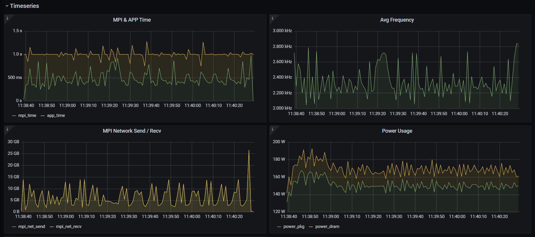
After understanding how Countdown works, I added all the data that needs to be sent from Countdown to the database using the MQTT protocol. Then it is possible to visualize the data in Grafana (an interactive visualization web application) by adding some plots :

Figure 1 : Example of dashboard

What’s next ?

Eventually I need to add a bunch of features in the Grafana dashboard to be more user-friendly and complete

If you were to investigate the interaction of two atoms, where would you start? Let’s start thinking of the most uncomplicated atom, Hydrogen. Well, the most fundamental thing we know about them is that they obey the Schrödinger equation. Here are the things that we need to take into account to solve the Schrödinger equation:

  1. Kinetic energies of nuclei
  2. Kinetic energies of electrons
  3. Electron-ion interactions
  4. Electron-Electron interaction
  5. Ion-Ion interaction

And they all are the functions of three spatial coordinates. It escalated pretty quickly… What if we want to examine the Tungsten atom, which has 74 electrons? It is impossible to solve such an equation without approximations!

Since approximations we make will affect some of the quantities of the outcome, we need to determine:

  • What do we want to learn about the system?
  • How large should the system be?
  • What time interval do we want to investigate?

There are a wide variety of models to describe the properties of atoms, molecules, materials, and rigid bodies. For example, Density Functional Theory(DFT) describes many-electron/many-body systems in terms of electron densities. It can be used to investigate the ground state electronic, optical, and chemical properties of materials in the picometer-nanometer range. However, it still is a quantum mechanical model, and the computational complexity of the systems increases with the cube of the number of electrons present in the system. DFT is practical up to a few nanometer scales but can provide a detailed description of the system.

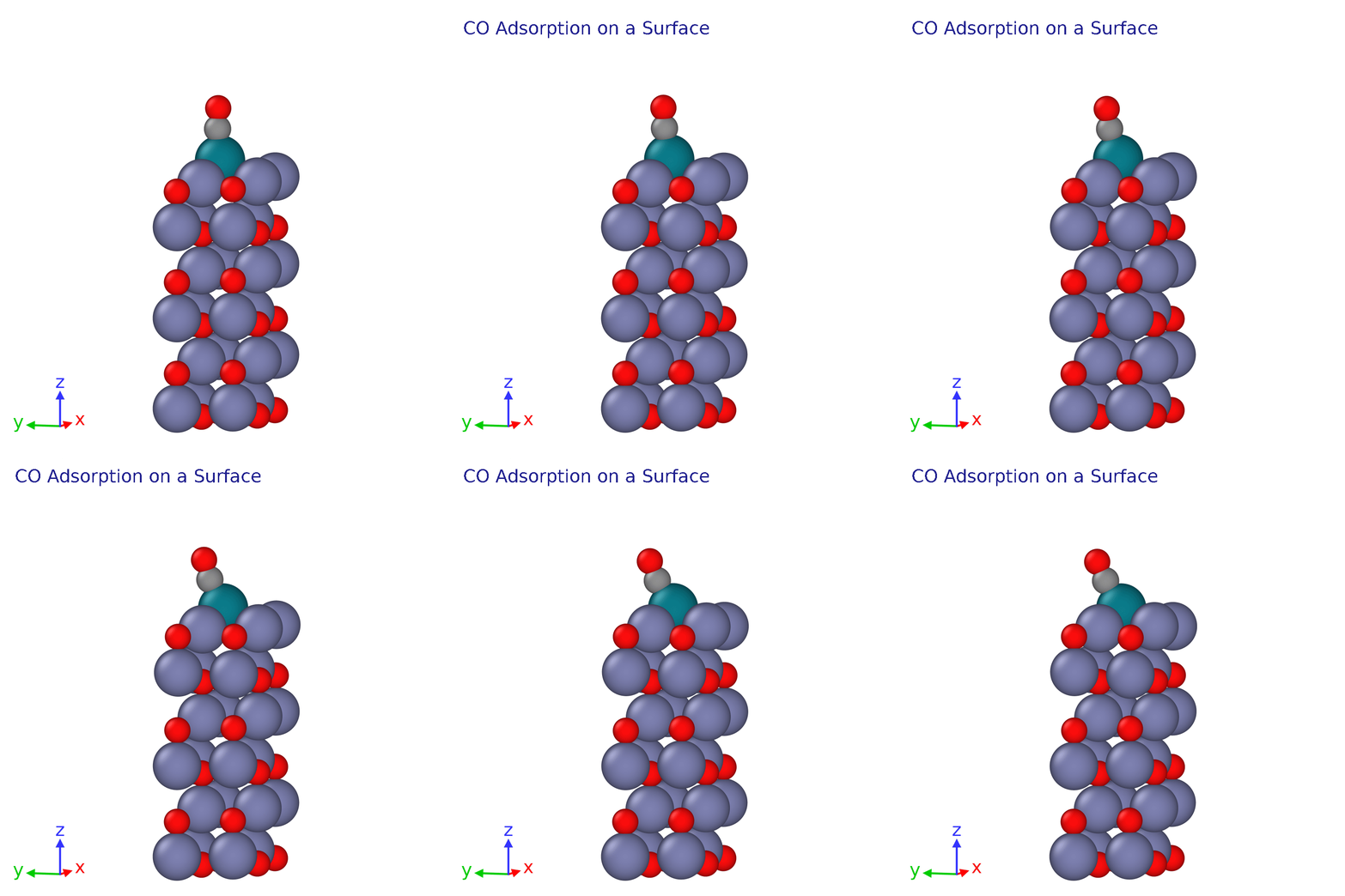
CO Adsorption Simulation with DFT

There is a more practical method called Classical Molecular Dynamics for larger and time&temperature-dependent systems. In this method, atoms are treated as point particles, and the interaction between them is described with the interatomic potentials. The time evolution of the atoms is obtained by solving equations of motion based on Newton’s Second Law! Moreover, the thermodynamical properties are controlled with statistical methods. With this model, systems with millions of atoms can be studied!
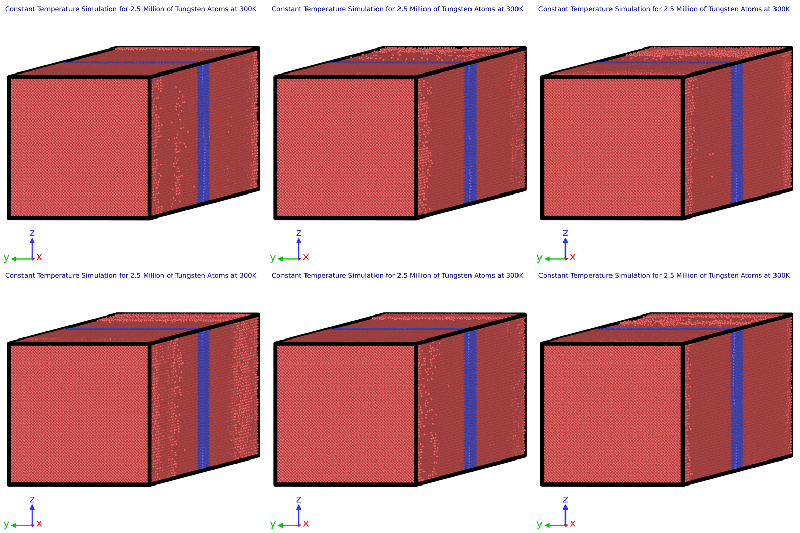
Constant Temperature Simulation with Classical Molecular Dynamics for 2.5 Million of Tungsten Atoms

Returning to the questions above, we want to investigate the thermal conductivity of irradiated Tungsten, which is one of the promising candidates that can be used inside Fusion Reactors because of its high melting point and endurance. The system should be large enough to simulate the damage caused by neutron bombardment and to observe a meaningful temperature gradient between the hot and cold regions. This means that we need to simulate more than a few nanometers. Finally, we want to study our system for pico-nanoseconds which is also vital for statistically valid thermodynamical properties.

In our study, we use Classical Molecular Dynamics, implemented in LAMMPS(Large-scale Atomic/Molecular Massively Parallel Simulator). The simulations contain 2.5 million atoms, and we are running them at Barcelona Supercomputing Center.

Okay, let’s put some context. I arrive in Nice and I have 2 months to develop and implement a few data post-processing routines in a plasma simulations code. The code currently stores files with data of thousands of particles that occupy an egg and the relevant information that can be extracted from there is not even a tenth of what it occupies, so my job is to perform the post-processing of that data within the code itself, so that its output is directly the information of interest. All good, all right.

Do you know how long it took me to start working on the post-processing routines? Almost a month! And you may ask: Julen, what have you been doing all that time? Easy. I’ve been understanding and fixing problems.

The first thing I had to do was to install the simulation code on the supercomputer where I would be working for the whole summer. Anyone who has ever done this process knows that this is usually a tortuous path full of incompatibilities and indecipherable error messages. But it was achieved.

Then we wanted to do some code scaling on this supercomputer. To put it quickly and badly: to see how long the code took to execute as we made it bigger and bigger (please, don’t kill me; if I’m not succinct, we’ll be here all day). You can’t imagine the headaches this brought, the behavior didn’t make sense! The code, with the same configuration, seemed to take random times to run.

How were the supercomputer nodes connected? What were their capabilities? What could be causing the erratic behavior of my code?

In the end we understood the behavior a little better: when I requested enough cores to have to make use of different nodes, the speed depended on the particular combination of nodes I requested to carry out my work. There seemed to be two branches: a fast one and a slow one, with consistent times in both cases. And why does this happen? Ah, who knows. It will be a mystery from now until the end of time.

By now it had been almost three weeks, between tests, research and, above all, many, many turns around the same thing. But it’s all right: let’s get to work.

The simulation code gives us the tensor of plasma pressures in different cells of the simulation box. We are interested in having the temperature tensor, and not in the code coordinates, but in local coordinates relative to the magnetic field direction.

Easy peasy. A little bit of formulation, a little bit of algebra, be careful with the units…

Everything seemed to work fine. What? Do you want me to put what I have calculated in a single file instead of having different files with the different components? Done.

Done? Difficulties come from where you least expect them. I had everything well calculated, but we wanted to save it all in a tensor form in a VTK file that we could open with paraview to visualize the data. This proved to be terribly problematic. How is the format correct? Why do I get everything right and the program doesn’t get the values right? Why is this all sooooo poorly documented? I just want to put in the numbers I have already calculated!

I have spent, I think, five times as much time trying to write things into files as I have calculating those things correctly.

I could go on telling you about my misadventures. I have implemented more routines and achieved interesting results. I will tell you about them in the last blog entry. But I didn’t come to talk about the results here. I came to talk about the process.

When you read about other people’s research and results, everything seems easy. We took this data, calculated that, and came up with these results. We wrote a program that did this and this, here it is… a lot of times you might wonder where all those months of work, all that time to do things that, a lot of times, don’t seem like such a big deal.

But that’s not the work. Research is hitting a wall over and over again, unable to find the door. Research is a labyrinth full of dead ends, where time and time again you have to retrace your steps. Even when you know exactly what you want to do, you can never imagine the problems that lie ahead until you actually do it. It’s spending hours and hours and hours and hours accomplishing nothing until you find the right way to do something and implement it in 10 minutes.

This may sound a bit disheartening, but there is a secret to this process. Learning. Every mistake, every unexpected problem, every little thing that you lose the whole day’s work to, is a learning experience. Do you know what I have learned about supercomputer architecture by scaling the code? What I have learned about data visualization and VTK format in my battle against writing data? Ooh, that’s what makes me now able to repeat what I’ve done all these weeks in a few days. Now I know more. But I know it because of all these little detours one encounters along the way. Those detours where we researchers spend almost all of our time.

So don’t get frustrated. Enjoy the journey. Even if you’re just going around most of the time. It may not feel like it, but you are moving forward. You are always moving forward.

As much as neural networks keep exhibiting their importance, featuring in the success records of several research works. Building good performing neural networks models do not come by easily due to some factors like finding the most suitable parameters for the model training, large size of data and computational complexities of the models.

Today’s briefing will be about a generic overview of how to improve the performance of model training. As discussed in the previous post, a deep neural network has the ability to approximate any continuous function. It is brilliant at finding the best relationship between features to produce the best results. Although, highly multidimensional data or high number of parameters tends to affect the performance of the model. In addition, having a large or deep model can affect the performance of the model too because it requires a lot of memory due to intensive computation. 

However, the advent of Graphics Processing Units (GPU) has come to unravel these caveats and makes it possible to conduct parallelization or distributed strategies for model training. GPUs process many pieces of data simultaneously which makes it useful for machine learning algorithms. Multi-GPUs demand communication among the processes and this is what brought about Message Passing Interface (MPI). MPI is a medium through which processes communicate. For instance, in point-to-point communication, two processors communicate directly between each other. While collective communication enables a single processor to communicate with several other processors.

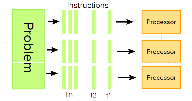
There are several strategies to carry out parallelism but we are going to be talking about just data parallelization and model parallelization in this post. Data parallelization is basically the use of the same model for every thread but with different parts of the data. While model parallelism is an act of using the same data for every thread, but split the model among threads.

A simple representation of parallel computing.

Lastly, these approaches have been good resources to build performant models of neural networks. Thanks for your time, but hope to see you again.

You may wonder how can we study and, more importantly, predict a material feature such as mechanical stability, thermal conductivity and so on. The answer is: solve the Schrodinger equation! Simple right? Right? … Well not that easy. The most complex system that we know how to solve exactly is the ionized hydrogen molecule. A solid system has billions and billions of atoms and electrons that is impossible to solve by hand. That’s why we use supercomputers. But there are many ways to solve the Schrodinger equation. One of the most used is Density Functional Theory ( DFT ). This method is based on the electron charge density and, without going into details, within some reasonable approximations, it allows as to know precisely all the dynamical, thermal, … In short all the properties of a material.
In my project “Heat transport in novel nuclear fuels” the supercomputer of Ostrava IT4Innovation National
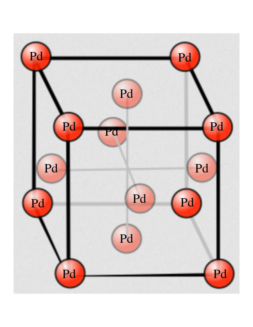
Supercomputing Center comes to our aid. I used the Vienna Ab-Initio Simulation Package (VASP) software module, that simply implements DFT, to look into the well known properties of palladium, as an exercise, that I now want to share with you. First of all let’s look at the structure of Pd. It is known as Face Centered Cubic (FCC) and it looks like this:

Other important features are the mechanical ones. How much can I stretch a solid? After what pressure it brakes? This features can be calculated “by hand” changing the input files. An important parameter of the structure of a solid is the lattice parameter (a) that is the side of the cube you see above. Changing it means to dilate the material and to see how the energy per atom (E) depends on it is related to the answer to the questions above. This E(a) curve determines the mechanical properties of the material.

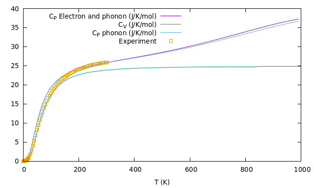
What about the thermal properties? There is a general one to one correspondence between temperature and vibrations of particles. The more particles moves the higher is the temperature. So, in a solid, it’s important to look at the motion of electrons and phonons (just a name for quantized vibrating nuclei motion). What it’s calculated is the so called dispersion diagram, i.e. the relation between the energy (or frequency) of a particle and its momenta. This is important to understand how many states are present at a certain energy (the Density Of States) and consequently all the thermal properties. An example of a theramel feature of a solid is the Heat Capacity at constant pressure, Cp, that, most importantly, is measured in experiments. Below I report what I computed on the supercomputer versus some experimental results as an example of the great reliability of DFT.

Graph of Cp with different contribution (electron and phonon) compared with experimental measurements.

In the next weeks me and Luigi will investigate the properties of possibly the new generation nuclear fuels thorium and uranium sesquicarbide Th2C3 and U2C3. What is important in this study is to understand how the presence of carbon atoms in thorium and uranium compounds effect the heat transport feature. This will tell us if carbons increases or decrease the thermal conductivity (i.e. the efficiency) in a possible nuclear fuel. Anyway, thanks for your attention and see you next weeks! Hopefully we will update our blog soon with great results!

Is it possible to know the depth of the sea just with a photo? How?

Yes, it´s possible. This is what I´ve been researching this summer and I´m here to explain you how I did it.

Introduction

We call the maps of the depth of the sea bathymetric maps. Traditionally, these maps are measured taking sensors to the ocean, like vessel-based multibeam sonar or active non-imaging airborne lidar bathymetry. However, these methods used to be expensive in terms of time and money and in shallow waters they are even more expensive. For these reasons scientists could only map about the 20% of the ocean´s seabed.

For measuring the depth in shallow waters there is an innovative and experimental technique that uses only satellite images. This technique can only be used in shallow waters and its accuracy is limited by different factors like the satellite image pixel size or the water turbidity . So, as I said in the title, with just a satellite photo you can measure the depth of the seabed.

How do they do it?

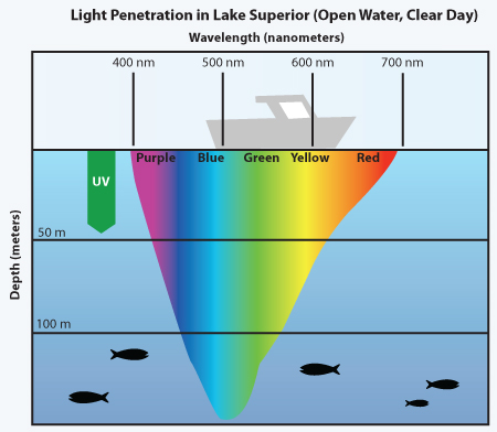
When sun light comes to the ocean, the different wavelengths are reflected in different proportions, and not always in the same way. Actually, ocean has not the same blue colour everywhere. Many factors like the impurities, the plankton, the turbidity or the depth, can change the spectrum of the sea. So, since depth is a factor that modifies the sea reflectance spectrum, it´s possible to study it just by looking at the water spectrum. In the visible spectrum range blue colour penetrates deeper in the sea than red or green. So, comparing the reflectance of the blue colour respect green or red we can get something called pseudo depth (pSDB) which is proportional to the real depth of the water. Figure 1 illustrates how different colours can penetrate into the water.

Figure 1 : Scheme of the visible light penetration depth into the water.

One way of look at the spectrum is using satellite data. In my case I used satellites Sentinel 2A and 2B that allowed me to study 8 bands in the visible and near infrared range, with a pixel size of 60x60m. I had two blue colour bands, one red and a green one, so I compared the two blue bands with the red and green bands obtaining a total of 4 pSDB combinations. If we know some real points in the area where we are working, we can convert this pSDB in a depth with a linear regression. I calculated the depth in North Adriatic and Calabrian Seas using more than 100 satellite images between 2020 and 2022. Then, I did an average of the calculated depths using those images where I got better results. That´s how I did the following bathymetric map of the shallow waters in the Calabrian coast.

Figure 2 : At the right we see the bathymetric map of the shallow waters in the Calabrian coast up to 20 meters depth. At the left we see the location of the study area.

On the next episode ….

Today we saw how I got bathymetric maps just comparing different colour reflectance bands from satellite images. On the next blog we will train an artificial intelligence to calculate bathymetric maps, we will study new band combinations and who knows, maybe I can discover something interesting.

Any comment or question it will be welcome.

See you on my next blog!


How are the materials made? How do electrons and ions arrange in a stable structure? Is your material a metal or an insulator? Is it opaque or transparent? Finally, is it a good nuclear fuel?

Density Functional Theory (DFT) is a computational quantum mechanical modelling method used to solve the microscopic problem starting from the charge density of our system. Electrons and Ions in a solid experience attractive interactions, electron-ion (negative-positive charges), and repulsive ones, electron-electron (negative-negative charges). Considering still Ions, interactions and focusing on charge density, it is possible to solve the electronic problem with DFT: given the crystal structure and number of valence electrons in a few second you will obtain the equilibrium distance and all the electrons available states, which ultimately determine the main properties of the material.

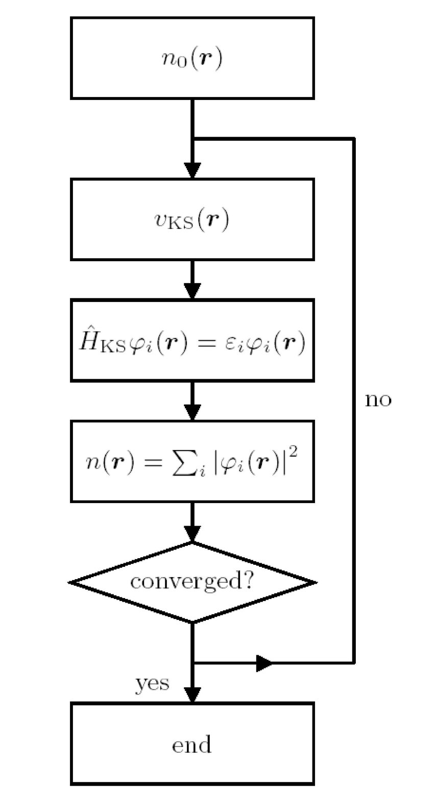
In the figure is shown the fundamental scheme of DFT self consistent algorithm. The starting point is a trial charge density that is used to calculate the Kohn-Sham potential, i.e. the potential experienced by all the other electrons in the solid. In the next step Kohn-Sham equation is solved that is nothing but a Schrodinger-like equation determined from a variational principle. If the calculated charge density is the same of the trial one then the algorithm converges and the problem is solved. Otherwise the calculated charge density becomes the input density and the cycle repeats.

In the previous weeks me and Mattia (the other guy engaged with me in the project ‘Heat transport in novel nuclear fuels‘ for IT4Innovations National Supercomputing Center at VSB – Technical University of Ostrava) worked on different materials, I studied Molybdenum, while Mattia Palladium, to understand the electronic and ionic physical property, e.g. the energy properties, the available electronic states, the structure stability, the lattice dynamics and the thermal properties. We have been working on the cluster Barbora with VASP (The Vienna Ab initio Simulation Package: atomic scale materials modelling from first principles) to run the DFT code, while we have been using Phonopy to understand the lattice vibrations (the so-called phonons).

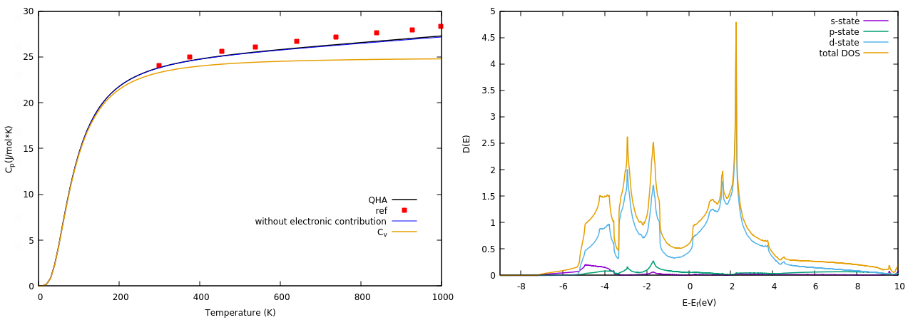
These are some examples of the quantities determined using DFT. On the left there is a thermal property, in particular the heat capacity at constant pressure considering both electron and phonons. On the right instead the electronic density of state, i.e. the number of available electron states per energy.

Over the next weeks we will be investigating the properties of the novel nuclear fuel. We will study the thermo-physical properties in thorium and uranium sesquicarbide (Th2C3, U2C3). In particular we will focus on how the presence of the carbon atoms affects the heat transport. If you are interested in the topic you can give a look at my next blog post, which will be focused on the procedure needed to calculate the main physical properties as thermal conductivity, heat capacity and thermal expansion that are fundamental properties in designing a new nuclear fuel. In any case, thanks for your attention and I hope you enjoyed this blog post.

So, what is Kokkos?

Modern high performance computers have diverse and heterogeneous architectures. For applications to scale and perform well on these modern architectures, they must be re-designed with thread scalability and performance portability as a priority. Orchestrating data structures and execution patterns between these diverse architectures is a difficult problem.

Kokkos programming model
The Kokkos programming model, broken into constituent parts. [Source: kokkos.org]

Kokkos is a C++ based programming model which provides methods that abstract away parallel execution and memory management. Therefore, the user interacts with backend shared-memory programming models (such as CUDA,OpenMP, C++ threads, etc.) in a unified manner. This minimizes the amount of architecture-specific implementation details a programmer must be aware of.

So, how is this done?

Kokkos defines 3 main objects to aid in this abstraction: Views, Memory Spaces and Execution Spaces.

Views: A templated C++ class that is a pointer to array data (plus some meta-data). The rank/dimension of the view is fixed at compile-time, but the size of each dimension can be set at compile-time or runtime. Each view also has it’s own layout, either column-major or row-major. This depends on which memory space the view stores it’s data on. (Eg: the host CPU, CUDA etc.).

The view dev allocated to the CUDA memory space. A shallow copy of the metadata is made from the default host space (CPU). [Source: Kokkos Lectures, module 2]

Execution Space: This is a homogeneous set of cores with an execution method, or in other words a “place to run code”. Examples include Serial, OpenMP, CUDA, HIP, etc. The execution patterns (such as Kokkos::parallel_for) are executed on an execution space, usually using the DefaultExecutionSpace, which is set at compile time passing the -DKOKKOS_ENABLE_XXX parameter to the compiler. However, one can change the space on which a pattern is executed as patterns are templated on execution spaces.

Memory Space: Each view stores it’s in a memory space, which is set at compile time. If no memory space is passed to the view, this is set to the default memory space of the default execution space.

This is only a very brief overview of the main concepts of Kokkos. A lecture series exploring these concepts and much, much more is available here.

What has been done so far?

The main aim of this project has been to explore the use case of Kokkos for Lattice Quantum Chromodynamics simulations, mainly developing staggered fermion kernels and comparing to handcrafted code for specific architectures. Working benchmarks of the staggered action and staggered Dirac operator have been developed. As Kokkos is based on shared memory, the current stage of development has been to extend these kernels to work on multiple nodes and GPUs using MPI.

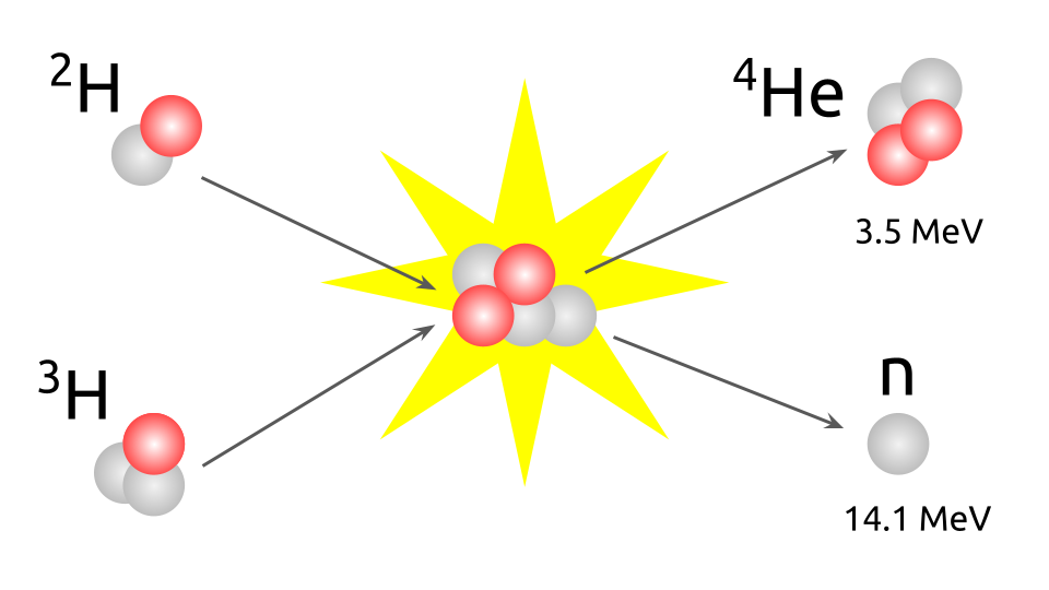
The deuterium-tritium fusion reaction. Red are protons, grey are neutrons. © Dominik Freinberger

My last blog post was devoted to giving an introduction on what molecular dynamics, the method I am working with this summer, is. In this post I want to talk more about the other side of the coin, the area of application of my project: Nuclear fusion and fusion reactors.


The Fusion Process

Nuclear fusion is the atomic reaction that makes our sun and the stars shine. It happens when two (or more) atomic nuclei come close enough together for the strong nuclear force to overcome the Coloumb repulsion between the protons in the nuclei. For certain (light enough) elements, this reaction is accompanied by a release of energy, as the fusion product is of lower potential energy than the individual nuclei as a whole. It is the difference in binding energy of the nuclei before and after fusion that is released. According to Einstein’s mass-energy equivalence E=mc2 the release of energy is equivalent to a mass defect, i.e. a loss of mass of the final nucleus compared to the individual initial nuclei.

The promising fursion of deuterium and tritium. © Dominik Freinberger

In our sun hydrogen nuclei 1H fuse into a helium core 4He in a multi-stage process known as the proton-proton chain. The most promising fusion partner candidates on earth are the hydrogen isotopes deuterium 2H and tritium 3H by means of their fusion reaction rate relative to energy input in terms of temperature. Deuterium-tritium fusion produces a helium nucleus and a free neutron, accompanied by 17.6 MeV of kinetic energy of the resulting particles. With 14 MeV, the neutron carries the lion’s share of the energy, which has to be converted into practically usable energy.

While millions and millions of tons of hydrogen fuse into helium every single second in the sun, releasing an enormous amount of energy as a result, this process is not so simple to replicate on Earth. In the Sun and other stars, besides the high temperatures and high density, it is the enormous gravitational pressure that brings the atomic nuclei close enough together for a long enough period of time to overcome (actually tunnel through) the Coloumb barrier and allow the nuclear forces to take over and enable nuclear fusion to occur.

Since it is not possible to realize such pressures on Earth, the fusion fuel must be brought to even higher temperatures than in the core of the Sun – tens to hundreds of millions of degrees Kelvin. At these temperatures, electrons and atomic nuclei are separated from each other and form an electrically conducting plasma. Additionally, the plasma must be confined as in the Sun to resist expansion due to it’s own pressure. Since no material on Earth can withstand these temperatures and the plasma would cool down immediately if it touched any wall material, the plasma must be controlled in a very special way. Arguably the most well known and best researched approach to this is magnetic confinement as implemented in a Tokamak or Stellarator reactor. Both concepts exploit the fact that charged particles in a magnetic field experience Lorentz force and follow helical paths along the field lines. In both designs, the plasma is kept floating in a vacuum using strong external magnetic fields. As my project deals with studying properties of parts of the first reactor concept, the Tokamak, I will discuss this one in more detail.


The Tokamak Reactor

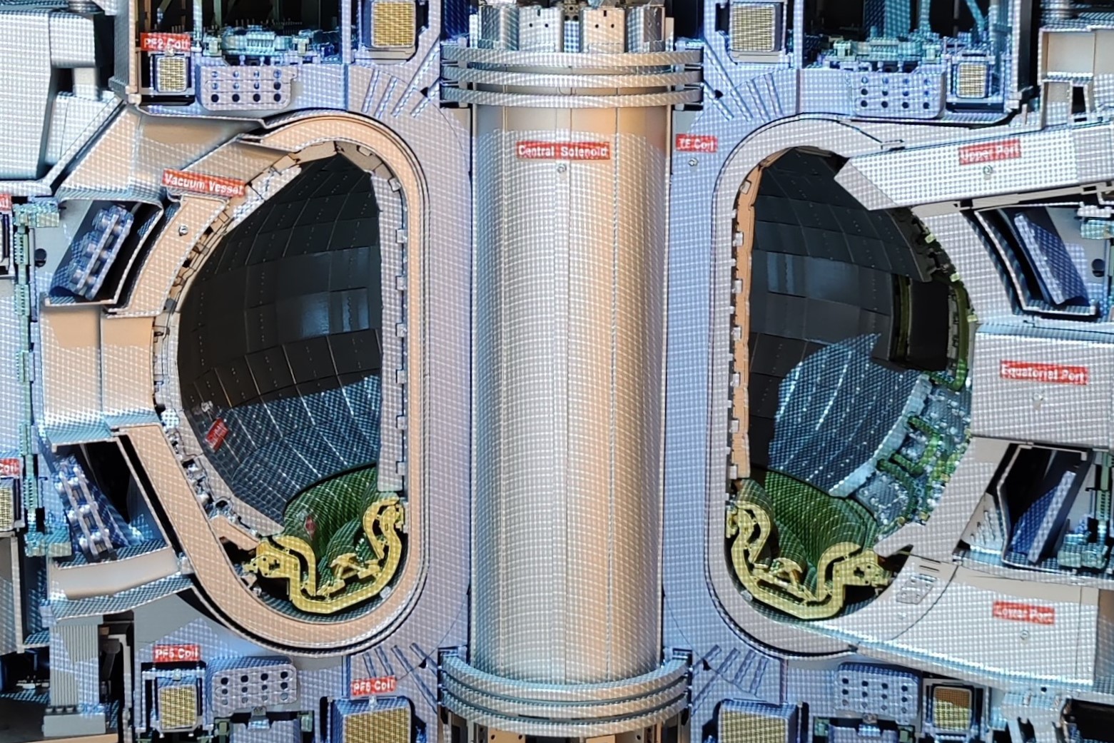
Model of the ITER Tokamak at the ITER facility. © Dominik Freinberger

The term Tokamak originates from the Russian word токамак which is an abbreviation for toroidal’naya kamera s magnitnymi katushkami – meaning toroidal chamber with magnetic coils.

The name says it all: The Tokamak is composed of a toroidal chamber (doughnut shape) which is surrounded by torodial magnetic field coils. These magnets provide for the confinement of the plasma. In addition, a central magnet, the solenoid, induces a strong electric current in the plasma itself, which serves to stabilize the plasma. This principle can be compared to a transformer where the plasma acts as the secondary winding. Another set of poloidal field coils is used for positioning and shaping the plasma.

An important component of future tokamak reactors is the divertor. It is located in the lower part of the plasma chamber and is used to remove “fusion ash” – helium, unburned deuterium and tritium as well as impurities – from the fusion plasma. Parts of the divertor are so-called plasma facing components and are therefore exposed to particularly high radiation loads. One candidate material for this application is tungsten, which I am investigating in the course of my project to determine how its thermal conductivity is affected by irradiation.


ITER

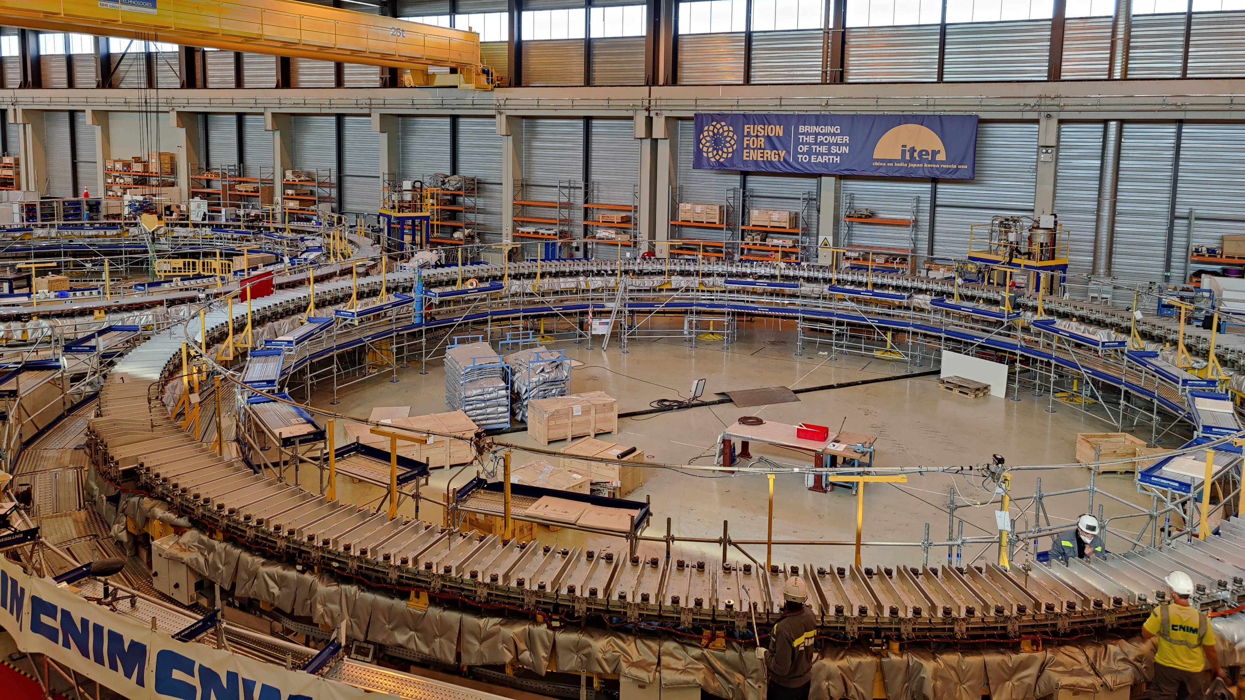
On-site construction of the poloidal field coils at the ITER facility. © Dominik Freinberger

Finally, I would like to mention a particularly impressive example of a tokamak: ITER – International Thermonuclear Experimental Reactor. Currently under construction, this massive collossus of a fusion reactor is being built in the south of France, at the Cadarache nuclear research center. In a few years, the first plasma is to be ignited here, ultimately proving the feasibility and economic viability of nuclear fusion. ITER is an unprecedented international collaboration on a global scale.

In September 2021, I had the unique opportunity to participate in a guided tour to the ITER site. The picture above shows the on-site construction of the aforementioned poloidal field coils – to give an idea of the scale of this project.

Just as the first plasma will soon be ignited in ITER, I hope this post was able to spark some interest in nuclear fusion.


Teleportation might seem a fancy expression and you might think it’s only possible in fictional world. However, it’s the reality in quantum communication. No quantum information is actually being transferred between sender and receiver during the process except the must needed classical data which is sent through a classical channel.

What is quantum teleportation? 

If you already read my first blog, I promised to come back again with my first month’s experience of the HPC project. By this time, I have learned two important algorithms and one protocol as an initial training. It’s quite hard to talk about all of them in this short context, so I chose to give you a quick go through about the quantum teleportation protocol. 

Quantum teleportation is basically a protocol that facilitates the transfer of quantum information i.e. an unknown quantum state,


from sender to receiver. Say, the sender is named Alice and the receiver is named Bob, then the information transfer between them requires two main components:   

  • A source to produce an entangled qubit pair or EPR pair.  
  • A classical communication channel to transfer classical bits. 

In case you are unfamiliar with the concept of the entangled state, it’s a quantum state such as,


Clearly, this state has a 50% chance of being measured in the state |00⟩ and a 50% chance of being measured in the state |11⟩. The most important implication of such a state is that measuring one qubit will tell us the state of the other as the superposition collapses immediately after measurement. For example, if we measure the top qubit and get the state |1⟩, the overall state of the pair would be:


Why such implication is significant for quantum teleportation is the fact that, even with a separation of light-years away, measuring one qubit of the entangled pair appears to have an immediate effect on the other. Now let us focus on the protocol itself. A schematic is presented below.  

So you can see, both Alice(Source) and Bob(Destination) receives an entangled qubit pair (AB). Alice then performs some operations(Bell state measurement) on her end and sends the results to Bob over a classical channel. Upon receiving the classical information, Bob then performs some more operations on his end and finally has the state D. Let’s now look more closely what’s happening in each box. 

What’s inside the black boxes? 

We will now build the quantum circuit for the protocol in step-by-step. The fundamental components for any quantum circuit are quantum gates. Our protocol needs four single-qubit gates, which are, Hadamard gate, CNOT gate, X gate and Z gate. I would suggest you to look here to know more about quantum gates.

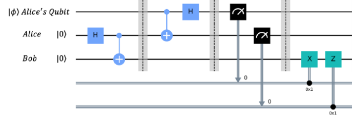
Quantum teleportation circuit using qiskit [Credit: Source].

Let’s go through the following steps and see how the circuit is built.

Step 1: The first step is to create an EPR pair of the qubits of Alice and Bob. It is done before the first dotted barrier by applying a Hadamard gate followed by a CNOT gate.  

Step 2: In this step, Alice applies two gates (CNOT followed by a Hadamard gate) on both the state |φ⟩ and her own qubit. For the application of CNOT, |φ⟩ acts as control qubit and Alice’s qubit acts as target qubit.  

Step 3: Now Alice applies measurement on both the qubit to be transmitted and her own qubit. She then stores the outcome in two classical bits and send them to Bob through classical channel. 

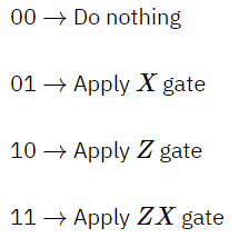
Step 4: Depending on the classical bits Bob receives from Alice, he now applies following operations on his qubits: 

And finally!! The state Bob receives is exactly the one Alice had. And that’s how the protocol enables a piece of quantum information to be sent to a distant receiver. If you are further interested about the mathematical proof whether the state Bob receives is the same state |φ⟩ or not, you can give this a read. 
 
I hope you learnt something interesting. Please do let me know in comments if you have any questions. I am yet to talk about my findings for this project. So, check my upcoming blogs if you want to learn more exciting stuffs about quantum algorithms.  

Antiviral Drug Development with MM-PBSA Calculations

This SoHPC Project aims to carry out HPC based Computational Screening for novel variants of the TAT-I24 peptide with improved binding affinity to ds-DNA.

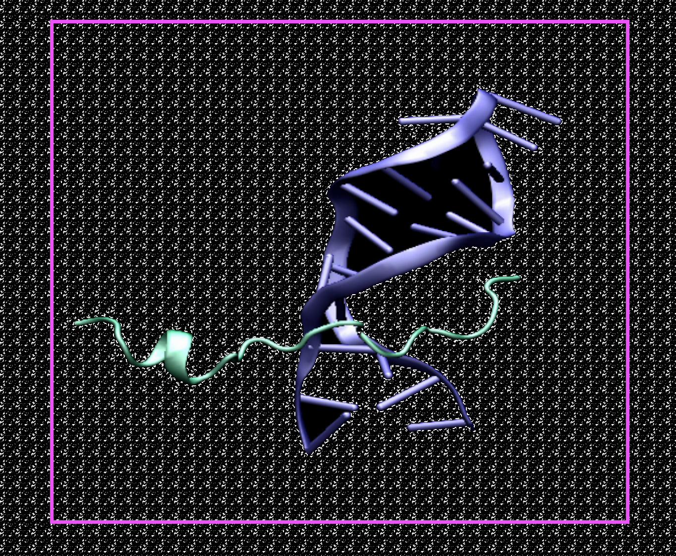
Figure1: Structural representation of the complex between ds-DNA (purple) and the TAT-I24 peptide (white, magenta) as revealed from MM/PBSA analysis with derived binding free energy of -36 kcal/mol.

The antiviral peptide targeted in our project is TAT-I24. The peptide TAT-I24, composed of 9-mer peptide I24 and TAT (48-60) peptide, exerts broad-spectrum antiviral activity against several DNA viruses. This peptide inhibits the replication of a large number of various double-stranded DNA viruses. Including Herpes Simplex Virus, Cytomegalovirus, Adenovirus type 5, SV40 Polyoma virus and Vaccinia virus. It aims to influence the activation of the virus by changing the amino acids of the proposed peptide and producing new variants. To further support this model, the current study explores the DNA binding properties of TAT-I24.

At the molecular level, direct binding of the peptide to viral ds-DNA can be observed. Consequently, the next simple step to further increase drug efficacy was to change any of the 22 amino acids and examine the effect of enhanced or impaired binding strength. Regarding the methods, the MM/PBSA technique can be applied. This computational approach allows semi-quantitative estimates of binding free energies (∆G) based on molecular dynamics simulations (MD).The molecular mechanics/Poisson-Boltzmann surface area (MM/PBSA) method is frequently used to calculate the binding free energy of protein-ligand complexes, regularly balancing the computational cost with attainable accuracy. The relative binding affinities obtained with the MM/PBSA approach are acceptable, but often overestimate the absolute binding free energy.

I need novel I24 variants to interact with TAT

The TAT-I24 peptide is the medicinal compound chosen in this project. It consists of the following 22 amino acid sequences, GRKKRRQRRRPPQ-CLAFYACFC. Ideally, we would test each position with the full set of 20 possible substitutions, so 2022 = 4.194304 × 1028 variants. However, individual computational connection free en-
energy calculations are absolutely inaccessible. What can be done instead is to randomly select a particular amino acid in the original sequence and replace it with another (randomly selected) and help calculate the resulting binding affinity of this newly modified peptide. MM/PBSA approach (doi:10.1021/ar000033j). In this way, at least some clues can be obtained about certain key positions in the TAT-I24 peptide that cannot be changed without compromising affinity for the target DNA. Choosing a clever strategy to substitute amino acids could reveal valuable insights into the denova design of an enhanced TAT-I24 peptide with increased activity against viral DNA.
The MM/PBSA approach has been shown to agree very well with the experimentally determined binding constants for the target system.

                           MD Simulations TAT-I24 in AMBER 

MD simulations and experimental protocols before MM-PBSA take time (approximately 2-3 days). For this reason, computational systems that perform as fast as possible are needed when calculating MM-PBSA.

If there is one with more speed when doing MM-PBSA :

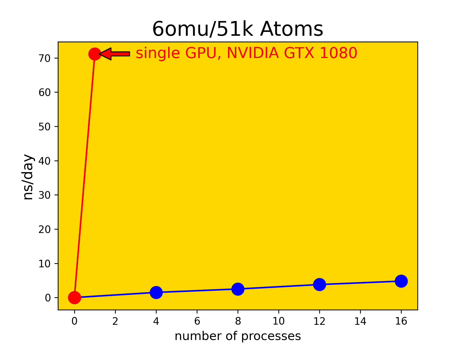
Figure 2: AMBER/20 benchmark for MD simulations of the 6OMU.pdb in explicit water (≈51k atoms). Blue dots are MPI parallel runs and the red dot is the achievable performance using a single GPU. Thus for the computational activity needed in this project (many 250ns MD simulations of randomly changed sequences of the TAT-I24 peptide) the GPU offers sufficient compute performance.

Thus we first need to establish a certain baseline of compute performance to appropriately plan and design the upcoming series of amino acid substitutions in the TAT-I24 peptide. To this end we chose an unrelated system (protein 6OMU.pdb in ex- plicit water) and carried out MD simulations with AMBER/20 using different parallel implementations. The idea was to compare conventional MPI parallel runs on CPUs to the performance available on GPUs. In this context SLURM submission scripts were set up and a series of parallel jobs was run using increasing numbers of CPUs in MPI parallel mode. The MD characteristic performance metric (ns/day) was obtained for each of these runs and plotted as function of numbers of processes (see blue dots in Fig. 2). This was then com- pared to the GPU performance avail- able on a single device of type NVIDIA geforce gtx1080 (see red dot in Fig. 2).

After comparing GPU and MPI performance, a Benchmarking was created for the experiments (with reference from previous experiments). In this way, MM-PBSA experiments are continued using GPU. In this way, more results will be obtained in a shorter time within the scope of MM-PBSA experiments using HPC.

N body simulations are fundamental in many areas of research. For example, if we want to predict how galaxies evolve or how molecules interact with each other you have to compute the Gravitational or Coulomb interactions.

Computational complexity

The first problem with these N-body simulations is that the naive approach has O(n2) complexity as it considers every pair of particles. To solve this we can use the Fast Multipole Method, bringing the complexity down to O(n). The algorithm exploits the fact that these interactions decrease rapidly with the distance among particles.

Another important feature is that its keeps the error bounded, and given the peculiarities of floating-point arithmetic it can even get more accurate results than the naive approach in some specific situations.

Exploiting supercomputer’s hardware

Once we have a good FMM implementation the next step is to parallelize it using constructs such as threads, tasks to be executed independently or even accelerators such as GPUs. This works great and has given good results concerning efficiency and speedup, but it has a big problem: you can’t scale! Scaling is important because we want to simulate increasingly complex scenarios, so we have to figure something out.

We can solve this issue with MPI, but doing so requires very hard work because we have to explicitly distribute the workload between nodes while keeping the number of communications to the minimum.

It is definitely a challenge but we’ll do our best! I hope you enjoyed the post and thank you for reading.

It goes without saying that the physics of an earthquake is complicated. This, in combination with the complex structure of the earth’s crust, makes the effects of earthquakes difficult to predict. Luckily, high performance computing and numerical models are the perfect tools to simulate complex earthquake scenarios!

In my first blog post I briefly mentioned that I would work on this project – an HPC wave propagation solver called SEM3D. This software is developed at my host institution and efficiently solves the 3D wave-propagation problem using the Spectral Element Method (a type of Finite Element Method) together with a time-stepping algorithm.

So far so good, but how does this actually work? In this blog post, I will try to summarize my first few weeks of learning, and hopefully give a good high-level explanation of how earthquakes can be simulated in an HPC environment!

Note: The Finite Element Method (FEM) is a popular method for solving differential equations numerically by splitting a large domain of interest (such as the earth’s crust) into smaller, simpler elements (for example cubes). The solution to the differential equation is then approximated by simpler equations over the finite elements. In this blog post, I will assume that the reader has some basic knowledge of FEM and numerical methods for solving (partial) differential equations.

Semi-Discretization of the Wave Equation

The wave equation is a time-dependent second-order partial differential equation, meaning that in addition to the spatial variables, one must also take time into account. Anyone that has ever written FEM code is fully aware of the increased implementational efforts required when going from 1D to 2D, or worse, 2D to 3D.

Since we’re already working with a 3D domain (the earth’s crust), we will not treat time as the fourth dimension in our FEM code, but instead, opt for semi-discretization and a time-stepping scheme. This essentially means that we formulate the spatial dimensions of the equation as a FEM-problem, but express time propagation as an ordinary differential equation which can be solved with a simpler numerical time-stepping scheme.

Spectral Element Method

The Spectral Element Method (SEM) is very popular for simulating seismic wave propagation. Unlike the simpler finite difference method, it can handle the complexity of 3D earth models, while (for this problem) offering better spatial discretization, lower calculation costs, and a more straightforward parallel implementation than normal FEM.

SEM and FEM are very similar in many aspects – both, for instance, uses conforming meshes to map the physical grid to a reference element using nodes on the elements and basis functions. These are some of the key features that differ SEM from FEM:

  • SEM typically uses higher-degree polynomials for the vector fields, but lower-degree polynomials for the geometry (whereas FEM often uses the same lower-degree polynomials for both)
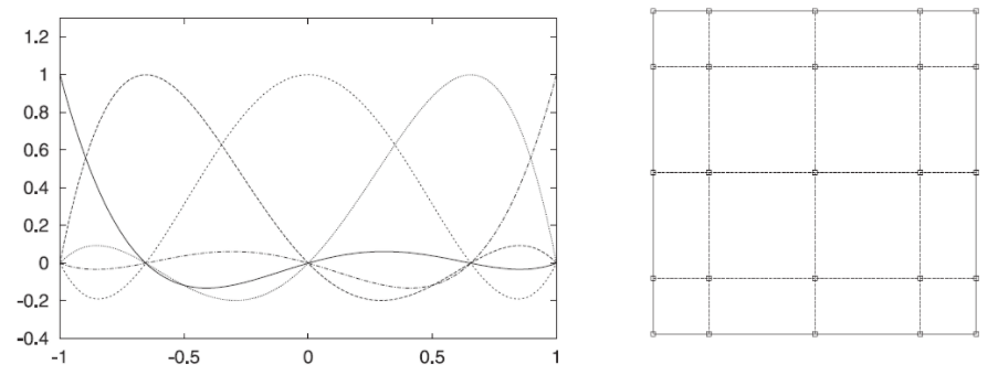
  • The interpolation functions are Legendre polynomials defined in the Gauss-Lobatto-Legendre (GLL) points (see figure).
  • SEM typically uses hexahedral elements in combination with the tensor product of 1D basis functions
  • For numerical integration, SEM uses the GLL rule instead of Gaussian quadrature. The GLL rule is not exact, but accurate enough.
Left: Lagrange interpolants in the Gauss-Lobatto-Legendre points on the reference segment [-1, 1].
Right: The (n+1)2 Gauss-Lobatto-Legendre points on a 2D face for n=4.

Although it may sound strange to limit the implementation to hexahedra, GLL points, and inexact integration, the combination of the three leads to an enormous benefit: a fully diagonal mass matrix. I really want to emphasize that this simplifies the algorithm and complexity drastically.

Time Stepping

After obtaining the mass and stiffness matrices M and K from the semi-discretization and SEM-formulation, we’re left with a second-order ordinary differential equation Mu”+Ku=F which allows us to propagate over time.

There exist several different time-stepping schemes, most of which are relatively straightforward. SEM3D uses a second-order accurate velocity Newmark scheme in which the velocity (u’) at the next time step is a function of the known velocity and displacement at the previous time step.

Stability

As in all numerical time-stepping schemes, stability (which depends on the time step, dt) is crucial. Since a large time step means less number of iterations and fewer calculations, we want to use the largest possible time step without losing stability. This is where I come in!

The classical CFL condition can be estimated for homogenous materials and structured meshes. When adapted to heterogeneous media, however, the method often becomes unstable. To avoid instabilities, SEM3D uses a safety factor which results in an extremely small time step, making propagation much slower than necessary.

The better alternative, and my job to implement, is an advanced stability condition based on the largest eigenvalue of the matrix M-1K. This advanced stability condition will allow us to calculate the maximum allowed time step without the safety factor, which means that the overall performance of the wave propagation solver will increase significantly!


That’s it for now – hopefully, you have a rough understanding of how seismic wave propagation can be simulated! In my next blog post, I will focus more on my own work and dive deeper into the implementation aspects of the advanced stability condition in Fortran 90 and an HPC environment.

As explained at the first post, my current project will make use of a supercomputer located at University of Luxembourg, called Aion which consists of 318 compute nodes, totaling 40704 compute cores, with a peak performance of about 1,70 PetaFLOP/s. This means it can 1.7 quadrillion arithmetic operations per second at its best!, but with that amount of computational resources one question arises, How could we take advantage of that amount of nodes?

Bash.. An old friend

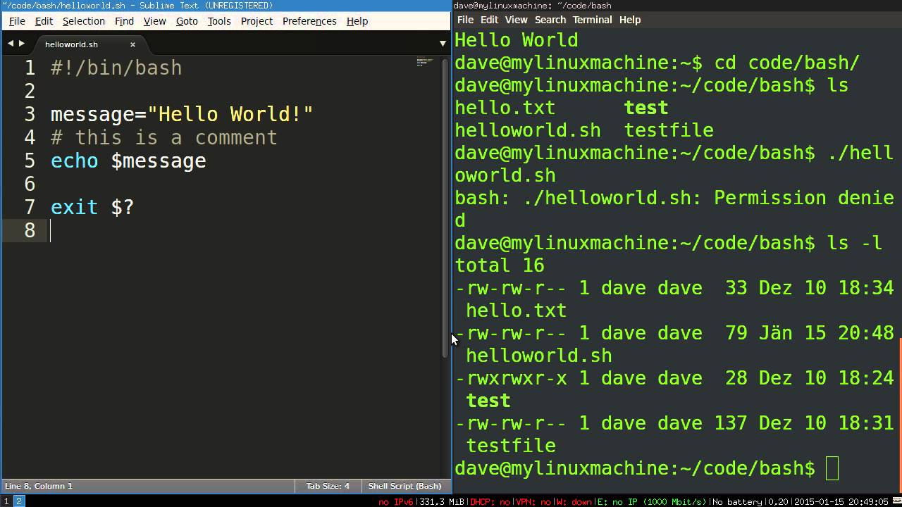
Before answering this question, let me introduce Bash, a command language which main task so to speak is to process the commands you give to it, from simple things as show “Hello world” on your terminal to complex scripts which manages several files. One example of usage is when you want to launch an specific executable, if you developed your own software you for sure want to test as soon as you finish it or in the meantime to see if it is working as intended, you can execute it in a bash script and make it suitable for your needs, do you want it to run thousand of time for different arguments or cases? No prob!, bash as well can manage for loops so you can automate this process.

One caveat for this is that only is planned to work for UNIX shells, the best known ones are MAC OS and LINUX, and guess what, more than 95% of supercomputers in the world uses LINUX ;).

Using the terminal and some bash will make you look like a hacker, just do not tell people that you are printing “hello world”

Communication breakdown

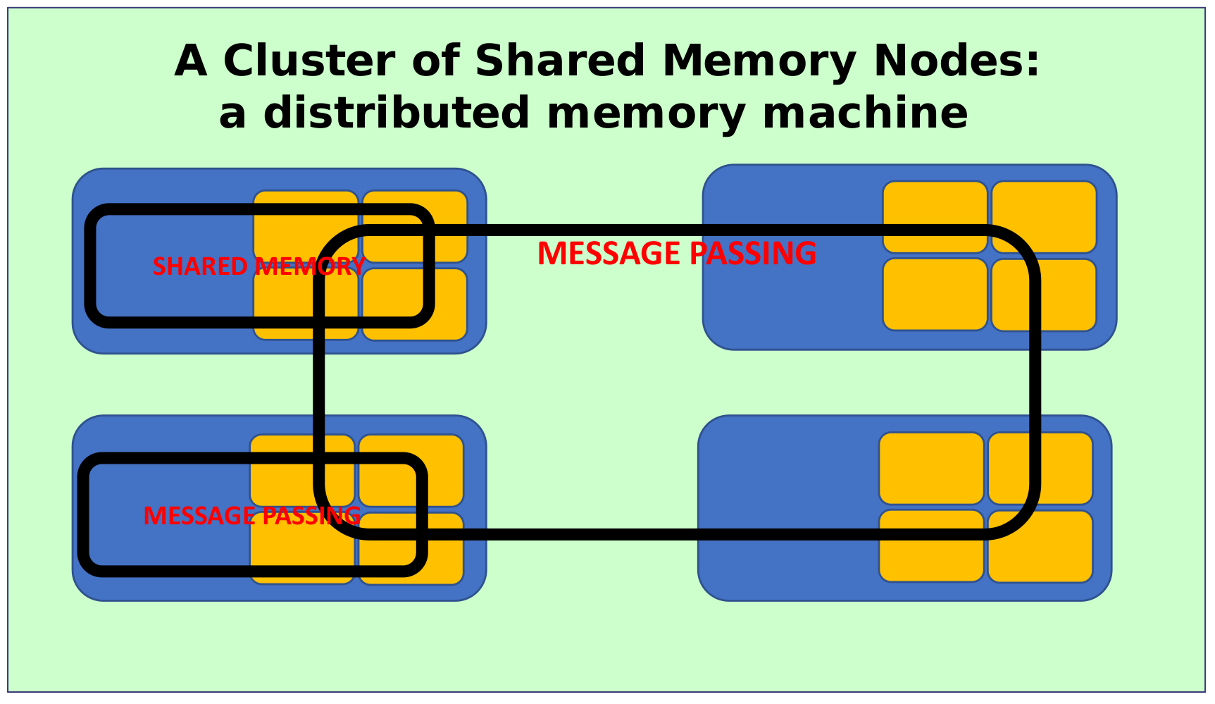
Alright now we have a tool that seems to do what we are looking for, but here is another caveat, each compute node we should consider as an independent resource and because of that if you want to make efficient use of every node available, they must communicate with each other in a smooth way!. Thankfully exists a network connection between every node called Fast InfiniBand (IB) HDR100 , you could send 100 Gigabit of data per second (theoretical peak) , almost like sending a FullHD movie per second to a neighbour node , not bad at all.

But we are not done yet, we still require a framework to manage the communication between compute nodes, and this is when MPI comes to play, a communication protocol framework available for different programming languages like C++ or FORTRAN, MPI sets how the data is structured , which message passing policy will be used, practically takes care of the communication back and forward between these nodes. Very useful as we said at the beggining that each node is independent, there is no shared memory between them , so there is no way that one node could access another node memory unless you use MPI.

As said before , each compute node should be treated as an independent compute, they can not share their memore unless by means of a message passing approach through network.

Now let’s automate .. right?

Do we miss something at this point? Seems like we have all the required tools to start but… normally a supercomputer is a shared resource between several departments and scientists and because of that, exists certain policies, priorites or amount of restricted resources available for each user. This supercomputer must contain a software that acts like a orchestra conductor, organizing the submitted jobs taking into account the priorities and policies, then scheduling the resources for everyone, in this case Aion uses a software called SLURM which will not let this supercomputer fall into anarchy :).

Now we know everything that is required to implement an automation for a performance analysis my friends, I am really eager to show you the final results for the next post, so stay tuned.

Generating random variables from an arbitrary distribution is a surprisingly difficult task, and Hamiltonian Monte Carlo (HMC) solves this challenge in an elegant way. Let’s consider a multivariate target distribution \pi(\vec{q}) , with parameters \vec{q}.

Elegant Animation of HMC Generating Samples from a donut-shaped distribution from Tom Begley’s Blog Post

Most Markov Chain Monte Carlo (MCMC) methods work by generating the proposals for the next sample (\vec{q}_{n+1}) from the current sample (\vec{q}_n). For instance, a MCMC method could take a random gaussian step in parameter space to get the next proposal. The proposal is then accepted or rejected with probability determined by the probability density at the current and the proposed positions. The rejection of samples at a lower density causes the walk to “stay on track”, and for computational resources to be focused on the typical set, where the density of the target distribution is significant.

This simple MCMC method struggles with high-dimensional distributions, as the volume surrounding the typical set is much larger than the volume of the typical set, meaning most propositions are in areas of low density and are therefore rejected. This isn’t very efficient, we can reduce the step-size to increase the acceptance rate, but this causes samples to be highly correlated.

This is where HMC steps in. Each point in the parameter space \vec{q} is assigned a potential energy u(\vec{q})=-\ln{\pi(\vec{q})}. To concretize this, image a 2D guassian distribution \pi(q_1, q_2) = \exp(-q_1^2-q_2^2). This has a bowl shaped parabolic potential energy function.

To go from one sample to the next, we give the “particle” a random momentum \vec{p} and simulate the evolution of the system for a certain number of time-steps. To concretize this imagine a hockey puck being given a random momentum in a large, parabolic bowl. In an ideal world, this method of generating proposals negates the need for an acceptance/rejection step, for reasons outlined in the references below. However, in reality, a small number of proposals are rejected due to numerical integration errors. Nonetheless, with a suitable time-step most proposals are accepted and samples have a lower correlation than those produced by simple MCMC.

Up until this point, Bruno and I have been working to implement and parallelize this algorithm with the help of our mentor Anton. In the next blog post I’ll talk about how we’ve been using jax, a python module which massively speeds up numpy on CPUs and GPUs.

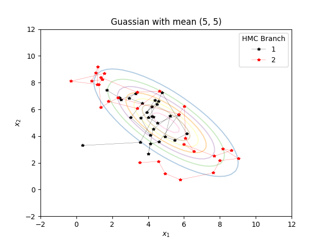
Two HMC chains exploring a potential. Each chain runs on a different CPU core.

References

Tom Begley’s Blog Post – Thanks for granting me permission to use the animation above!

M. Betancourt – A Conceptual Introduction to Hamiltonian Monte Carlo

It has been 6 weeks in the Summer of HPC and I realized I had not written a blog post that gives an insight into what we are doing. In this blog post, I would like to talk about the project’s purpose.

What is HiPerBorea?

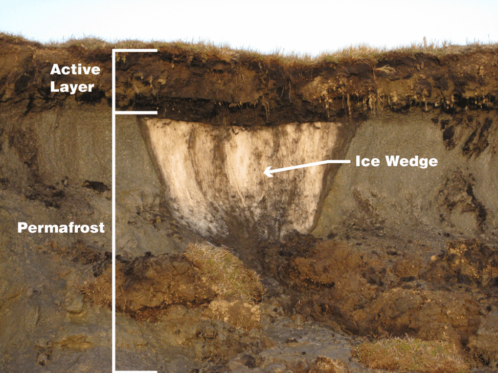
The project I am working on is titled HiPerBorea. The purpose of the project is to quantify the effect of global warming on permafrost areas, based on numerical studies at the watershed scale. You may ask, “What is permafrost?”. Permafrost is a thick subsurface layer of soil that remains below freezing point throughout the year, occurring chiefly in polar regions:

Permafrost

Unfortunately, due to climate change, these permafrosts are melting and causing severe impacts on our lives. For instance:

  • Many northern villages are built on permafrost. When permafrost is frozen, it’s harder than concrete. However, thawing permafrost can destroy houses, roads, and other infrastructure.
  • When permafrost is frozen, the plant material in the soil—called organic carbon—cannot decompose, or rot away. As permafrost thaws, microbes begin decomposing this material. This process releases greenhouse gases like carbon dioxide and methane into the atmosphere.
  • When permafrost thaws, so do ancient bacteria and viruses in the ice and soil. These newly-unfrozen microbes could make humans and animals very sick.

House sinking due to melting permafrost
(Credit kml.gina.alaska.edu)

What is permaFoam?

To quantify the effects of global warming, HPC tools and resources are needed. To satisfy this need, an open-source tool permaFoam, the OpenFOAM solver for permafrost modeling is built. This tool has been used intensively with 500 cores working in parallel for studying a permafrost-dominated watershed in Central Siberia and tested for computing capabilities up to 4000 cores. Due to the large scales to be dealt with in the HiPerBorea project, the use of permaFoam with at least tens of thousands of cores simultaneously is needed on one billion cells mesh.

We want to demonstrate that permaFoam has good parallel performance on big meshes which will be required to simulate actual geometries. To perform the scalability tests, we need to decompose the mesh into different processors. This operation is done by a utility in OpenFoam called decomposePar. However, it is working in serial and takes too much time and memory. Since we are dealing with more than 1 billion mesh, decomposing the mesh takes more than 1 week and more than 1TB of memory.

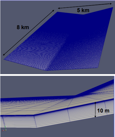
Mesh to decompose

We are developing a tool that does the exact same thing as the decomposePar utility does but in parallel using the domain decomposition method. After the tool is built, we will do some scalability tests which my partner Stavros will share the results with you.

I hope I made our aim clear and that you learned something from this blog post.

Thank you for reading.

For instance, the advent of self-driving cars like the Autopilot by Tesla, the Audi pilot driving system, speech to recognition, pixel recursive super resolution of video games, recommender system application from e-commerce like Amazon suggesting suitable products, to social media platforms like Instagram or Pinterest and also entertainment such as Netflix movies, Spotify musics, Youtube and the likes…

If yes, then I feel you might be curious to know the workings behind these stunning achievements. The success of these advancements can be ascribed to the concepts like Artificial Intelligence, Machine Learning and Deep Learning, thus stay tuned as I skim through the schema of these concepts.

To start with, the field of Artificial Intelligence (A.I) was formally founded in 1956, at a conference at Dartmouth College, in Hanover, New Hampshire where the term ‘’Artificial Intelligence’’ was coined. A.I is the science of getting machines to mimic  the behavior of humans or any living entity. However, Machine Learning (ML)  is an application of A.I where a computer learns from past experiences (inputs data) and adapts to become more accurate at making future predictions without following explicit instructions. The performance of such a system should be atleast at human level.

How does the machine learn and carry out predictions…?

In order to perform any task, ML provides various techniques that can learn from and make predictions on a dataset. Most of them follow the same general structure as seen in Figure 1 below.

Figure 1: The Structure of Machine Learning Models

The ML process starts with inputting training data into the selected algorithm, the system analyzes the pattern in the data, by understanding the relationship between the features and the targets, thus develops a learned model based on this. Afterwards, another dataset (testing data) is fed into the learned model to evaluate its performance. This process might be repeated multiple times until a desired level of performance is achieved, then the model can be used to make predictions on unseen datasets. There are several algorithms that can be used for the data modeling which depends on the use case, most of which are categorized as in Figure 2 below.

Figure 2: Classifications of Machine Learning Models

Unsupervised Learning

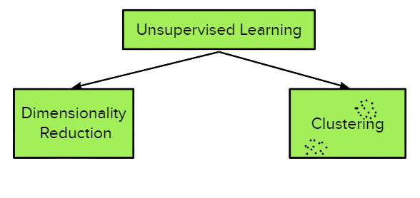
The concept of recommender systems earlier talked about is actually one of many applications of unsupervised learning. An unsupervised learning is a type of ML in which the models are trained using an unlabelled dataset and are allowed to act on that data without any supervision. The task here is to discover interesting attributes about the data without knowing the true answer. And it is divided into two parts as seen in Figure 3 below.

Figure 3: Categories of Unsupervised Learning

Supervised learning:

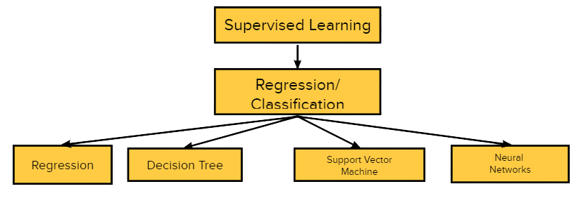
Conversely, Supervised learning is defined by its use of labeled datasets to train algorithms that are used to classify data or predict outcomes of an instance with a level of accuracy. The Figure 4 below explains its divisions.

Figure 4: The Flow Chart of Supervised Learning

Furthermore, building realistic and natural driving behavior, predicting what other cars might do in the next second, making decisions and few other features of self-driving cars we discussed earlier are puzzle pieces of deep learning which leverage the concept of supervised learning.

What is Deep Learning….?

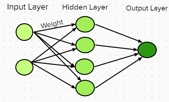
Deep Learning is simply the name used for stacked Neural Networks, that is, Neural Networks composed of several layers. Neural Networks are input and output systems with a layer structure. The machine learning process is inspired by the functioning of neurons in the human brain. Basically, it comprises of three major components that is; the input layer which propagates the input signal (features), the hidden layer which is made up of the computational units neuron (elaborating the signal from the previous layer) and lastly, the output layer that provides the final output signal all linked by weighted connection as seen in Figure 5 below.

Figure 5: A Simple Neural Networks Flow Diagram

Just like other ML models, the training, the evaluation and the optimization of the model to achieve a desired performance is the path to building any model. Obviously, this is just like an excerpt of fields involved in the success of the aforementioned advancements.

Lastly, the robustness of each field can not be overemphasized, for instance, the concept of neural networks have demonstrated outstanding performance in several research fields  to provide solutions to problems that seem complicated and which prompted the idea to leverage the concept to predict results of mechanical models in our ongoing project. In this project, we aim at investigating the ability of neural networks to approximate the results of mechanical models and their performance in terms of precision given some thresholds. The features of the dataset being used include parameters of the geometry, material properties, and applied forces while the target output is resistance or reserved factors. It is part of our objectives to explore different configurations of neural networks models and conduct hyperparameter tuning using different techniques to achieve the expected results.

For now, permit me to stop right here. I will keep you posted with the progress of the work, please stay tuned and feel free to share your comment in the section below…

Developing new drugs to act against COVID-19 is a current major necessity. Yet, before launching a new drug product into the market there are many steps that need to carefully followed, since the pharmaceutical industry is one of the most regulated industries in the world. First, a drug candidate needs to be discovered. Then, pre-clinical tests need to be carried out to evaluate the toxicity of the compound and to access its pharmacodynamics and pharmacokinetics. The next step is the clinical tests, in which the drug candidate needs to be tested in humans. Finally, the product needs to be launched in the market. All these steps can take up to 15 years. 

Drug development pipeline

A huge effort in the drug development pipeline goes in the pursuit for new drug candidates. In the past, this was done using an irrational approach by trial and errors, i.e., many substances are screened based on empirical observation.  Today, however, the pharmaceutical industry takes a rational approach, in which the drugs are designed to interact with the target of interest. To speed up the process and reduce the resources needed, computational techniques are being used to help engineering new drugs.

Among these computational tools, Machine Learning (ML) is getting much attention. ML is a technique in which the computer learns on previous experience. Based on the patterns found in the data from the system of interest, the algorithm creates models. These models can be used, for instance, to predict physicochemical properties of new molecules. They can also be used to predict drug-target interactions (DTI). Predicting DTIs is something that is of major interest in drug discovery, since it can be used to screen drug candidates.

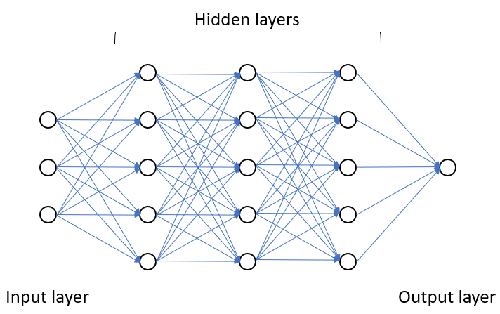
ML encompasses many different concepts, among them Neural Networks (NNs). NNs are based on the architecture of the brain and its neurons. In simple words, each neuron represents a mathematical function, called activation function. The neurons are grouped by layers, in which the output of all the neurons of a given layer goes to each of the neurons of the following layer.

Exemple of a topology for a Neural Network

Due to the COVID-19 pandemic outbreak on December 2019, the development of vaccines and medicines to be used against this disease ramp up rapidly. Many efforts have been made to develop a vaccine to protect the people from the SARS-CoV-2 virus. Yet, developing a medicine is also of great interest, as it can be used as treatment for people that already contracted the disease. 

In a previous work, Marián Gall and Michal Pitonák, the mentors of this project, used Neural Networks to predict docking scores of chemical compounds. The docking score is related to the biding energy between a chemical compound and a target, and is, therefore, a measure of the DTI.

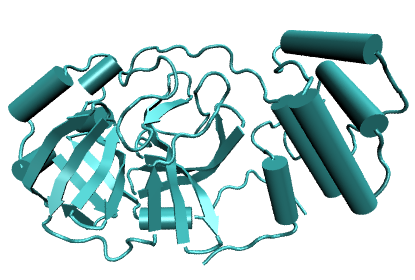
In our project we are also using AI to develop models to help the search for such drug candidates. These models are used to predict the interaction between a drug candidate and one selected target from the SARS-CoV-2 virus. This target is the 3CL protease, which is a protein related to the replication of the virus. Giving what has been done, the goal of the present project is to further develop the work of our mentors. The intention is to continue predicting the docking scores of chemical compounds, but also to develop new models that can have a better accuracy.

Representation of the 3CL protease

One of the challenges in dealing with computer techniques to model the properties of molecules is to represent them. Although there are different standard representations for chemical compounds, such as the IUPAC nomenclature, they cannot be used in ML techniques. This is because the molecules need to be represented in a way that the computer can interpret them, since it only works with numbers. Furthermore, the representation should be in a form that can be used as an input for NNs.

There are different techniques that converts the molecules from the form that we know into a representation that a computer can work on. These representations are also called descriptors. Example of descriptors are Coulomb Matrix, Atom-centered Symmetry Functions, Smooth Overlap of Atomic Positions, Many-body Tensor Representation, and many others. In their work, our mentors used the Smooth Overlap of Atomic Positions (SOAP).

In this project, however, we will explore other descriptors that are available. The new descriptors selected were the Coulomb Matrix, the Atom-centered Symmetry Functions, and the Many-body Tensor Representation. After obtaining the models using these other descriptors, the goal is to evaluate if one of them will result in better models than the SOAP.

Little bit of background

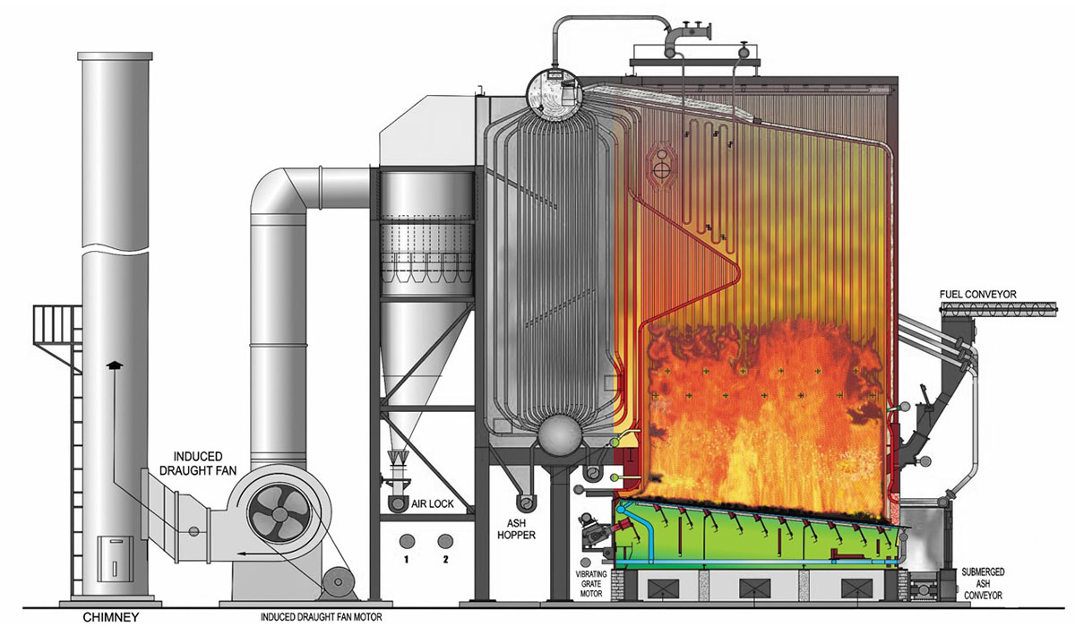
The data acquired for this project is from a biomass combustion simulation inside a furnace, this involves intricate physical phenomena and due to this complexity requires the use of High-Performance Computing (HPC) platforms.
In this simulation it is preferred to use a computational fluid dynamics(CFD) approach for gas simulation and a discrete element method(DEM) for the particles inside the combustion furnace, only CFD will not give individual or collective particle interaction and behaviour required to simulate chemical interactions and mass exchange with the surronding gas. CFD part is being carried by FOAM-extended (a variant of OPENFOAM for gases) and the DEM part by XDEM software as a numerical toolbox for the simulation of particulate material. Both software is coupled directly using C++ programmning language, that executes the respective parts of the simulation (CFD, DEM and coupling) allowing the two libraries to use the same memory and avoiding communication issues.

Imagine trying to simulate this whole process in a computer and get results close to real life, is not that awesome?

FOAM-extended is using a MPI-approach to parallelize the gas simulation and XDEM a OpenMP-approach, as particles usually lays on the fuel bed , it is mandatory that all those particle data belongs to only one MPI process so XDEM could only rely on multithreading. The way to decompose the CFD and DEM meshes is a crucial part to observe as it will determine a noticeable percentage of the total performance for the simulation. So for the next comparison we selected the simple decomposition which is a geometrical way to divide the furnace in geometrical blocks that communicate with each other and SCOTCH which is a OPENFOAM custom decomposition that detects and tries to spread the workload as balanced as possible.

Every plot should be an eye candy

All we should agree that data visualization belongs to the edge where art and science instersects, and it is really important to point out crucial information in a direct and easy manner to the final user. So for example you can show a bar plot of the different categories in your data, but are you sure that this plot will convey the main purpose of the information to the viewers? What about if there is a trend on this data , a pattern that is visible with the correct arrangement or geometry, or in the most of the cases, is it really easy for the viewer to understand and compare data in the plot?.

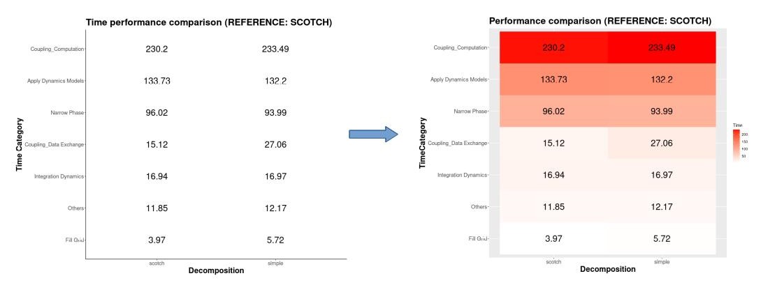
Let’s start with an example, a basic representation to show raw data directly would be a table, but let’s be honest, the brain is no trained to detect or do calculations with floating point numbers (if you can do this probably you would be very famous in a tv show), so it will be really hard for the viewers to compare changes in the data and even worse the magnitud of the change.

Could this be better right?

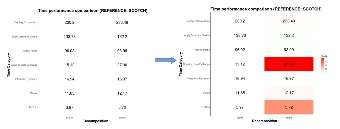
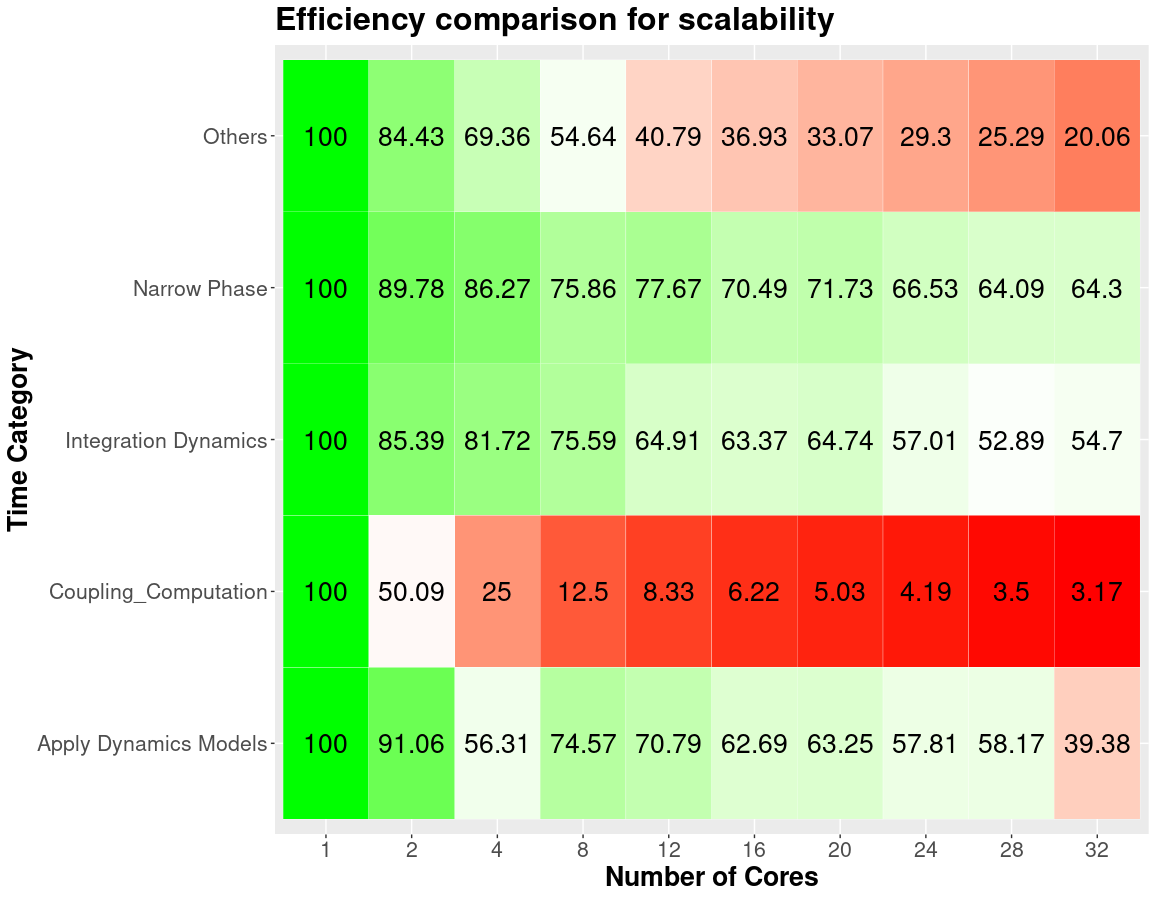
Taking in mind the figure above, we converted a boring table to a heatmap where it points the categories that takes the most of the time in the execution, but even with a heatmap would be really hard to compare between two different decompositions because we do not know which categories were impacted the most due to this new decomposition, so lets try to do a new heatmap but now we weight according on how much the time has changed in comparison with the previous one.

Now the heatmap points where are the biggest changes in time in comparison with the previous decomposition

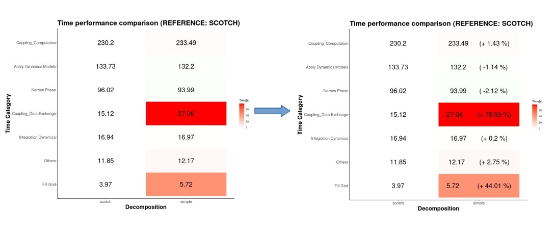
Now it is much better to see where the real changes occur, we can see that for the data exchange category occurs the biggest increment, and we can see that if the time decreases there is light green tone. But let’s make it more easy for the viewer, we are not human calculator so we will add the impact in terms of percentage.

Now we can see directly how much the categories have changed

And now with a single glance we can say that the data exchange category is the worst performant with a decrement of 78% with respect to the scotch decomposition. Could you do this with the raw table at the beggining?.

A language made for this

All of these is possible thanks to R, which is a programming language mostly present on statistics analysis and graphics, R is very well mantained and contains thousand of libraries implemented by developers around the world that make your life easier. In our case we used “tidyverse” as the most important package library, it allow us to extract transform and load the data present on our simulations, as well as a intuitive set of commands to manipulate the data structure to be more suitable for different kind of plots. Also it contains ggplot2 which offers a great variety of plots and graphs implementations according to the need to convey the right information to the viewer, as one of the most reliable sources to select the kind of plot suitable for our project was https://www.data-to-viz.com/. All of this along with the “here” package library which makes easy the file referencing as our data could be stored in different paths on the local storage.

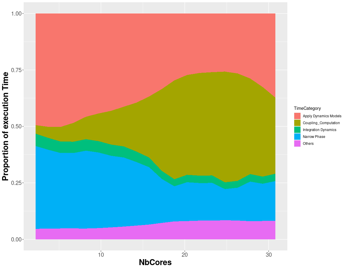
As we increase the number of threads, the coupling computation becomes a bottleneck

Follow by Email