
Project reference: 1717
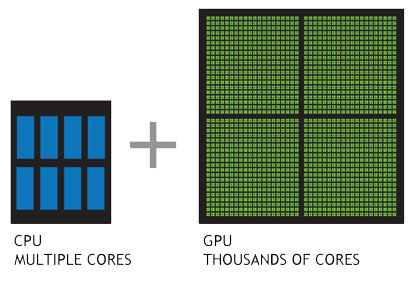
Today’s multi-core, many-core and accelerator hardware provides a tremendous amount of floating point operations (FLOPs). However, CPU and GPU FLOPs cannot be harvested in the same manner. While the CPU is designed to minimize the latency of of a stream of individual operations, the GPU tries to maximize the throughput. Even worse, porting modern C++ codes to GPUs via CUDA limits oneself to a single vendor. However, there exist other powerful accelerators, that would need yet another code path and thus code duplication.
The great diversity and short life cycle of todays HPC hardware does not allow for hand-written, well-optimized assembly code anymore. This begs the question if we can utilize portability and performance from high-level languages with greater abstractionpossibilities like C++.
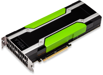
Wouldn’t it be ideal, if we had a single code base capable of running on all devices, likeCPUs (Intel Xeon), GPUs (NVidia P100, AMD R9 Fury) and accelerators (Intel Xeon Phi)?
With the help of AMDs open-source HIP framework (Heterogeneous-Compute Interface for Portability) it is possible to develop one code that can run on all hardware platforms alike.
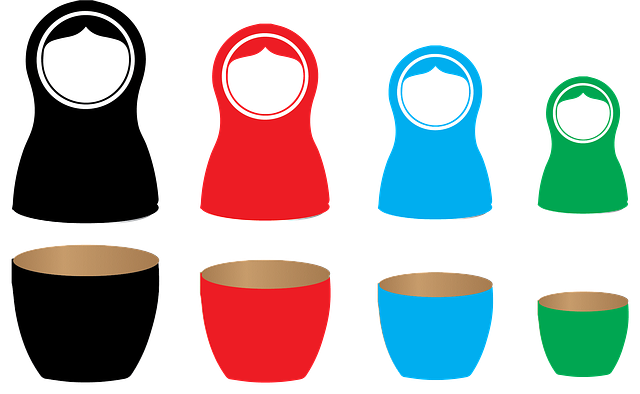
In this project we turn our efforts towards a performance-portable fast multipole method (FMM). Depending on the interest of the student, we will pursue different goals. First, the already availableCPU/GPU version of the FMM can be adapted to support HIP for the construction and efficient use of multiple sparse/dense octree datastructures. Second, a special (compute-intense) kernel for more advanced algorithmic computations can be adapted to HIP.
The challenge of both assignments is to embed/extend the code in a performance-portable way. This ensures minimized adaptation efforts when changing from one HPC platform to another.
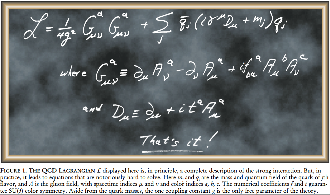
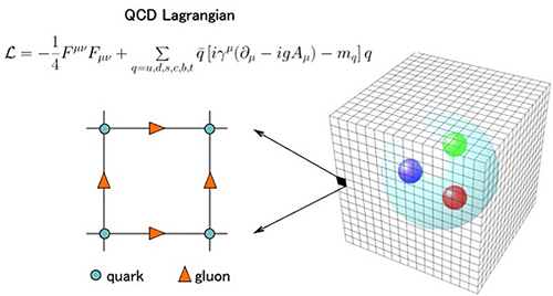
What is the fast multipole method? The FMM is used as a Coulomb solver and allows to compute long-range forces for molecular dynamics, e.g. GROMACS. A straightforward approach is limited to small particle numbers N due to the O(N^2) scaling. Fast summation methods like PME, multigrid or the FMM are capable of reducing the algorithmic complexity to O(N log N) or even O(N). However, each fast summation method has auxiliary parameters, data structures and memory requirements which need to be provided. The layout and implementation of such algorithms on modern hardware strongly depends on the available features of the underlying architecture.
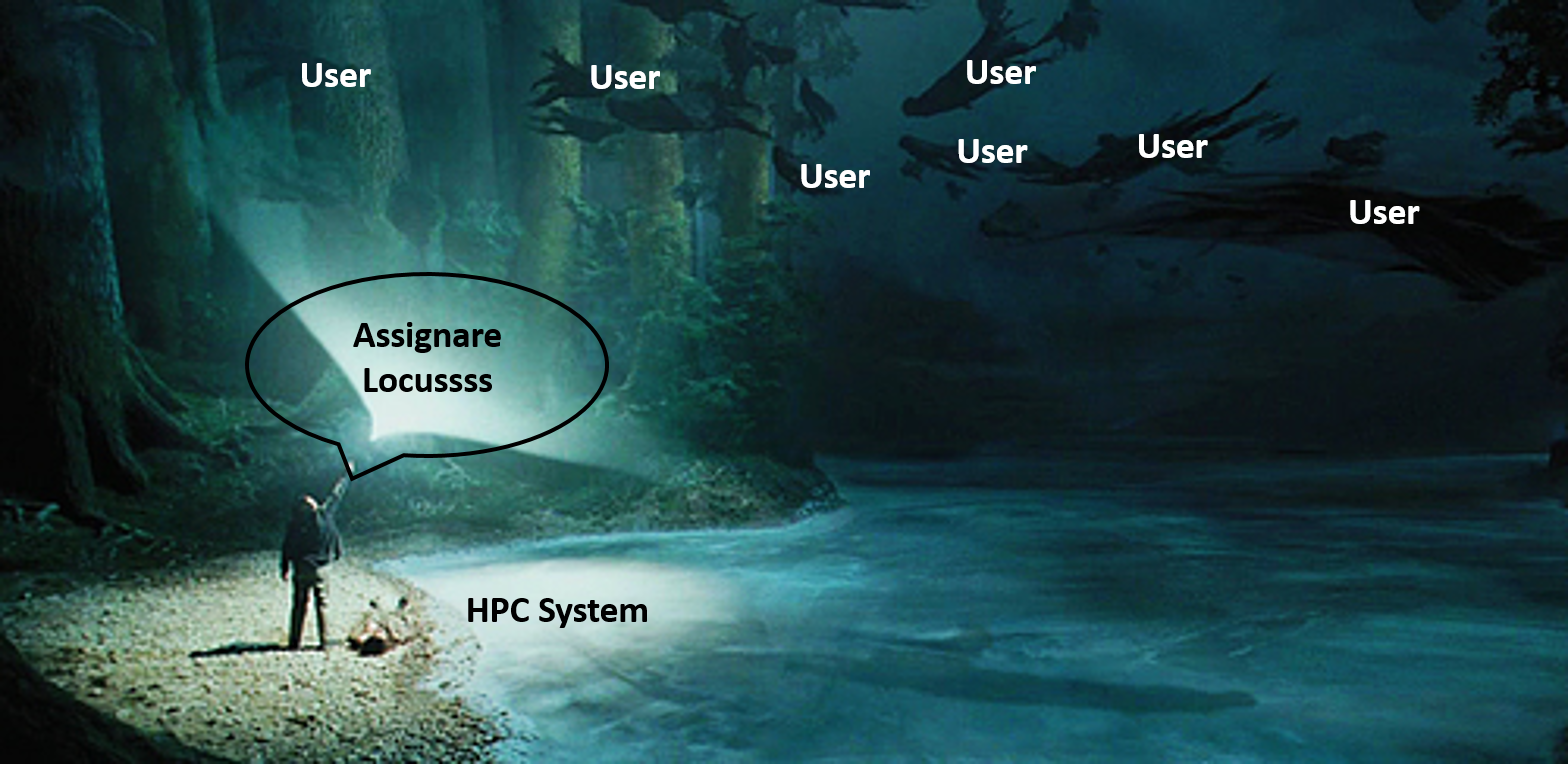
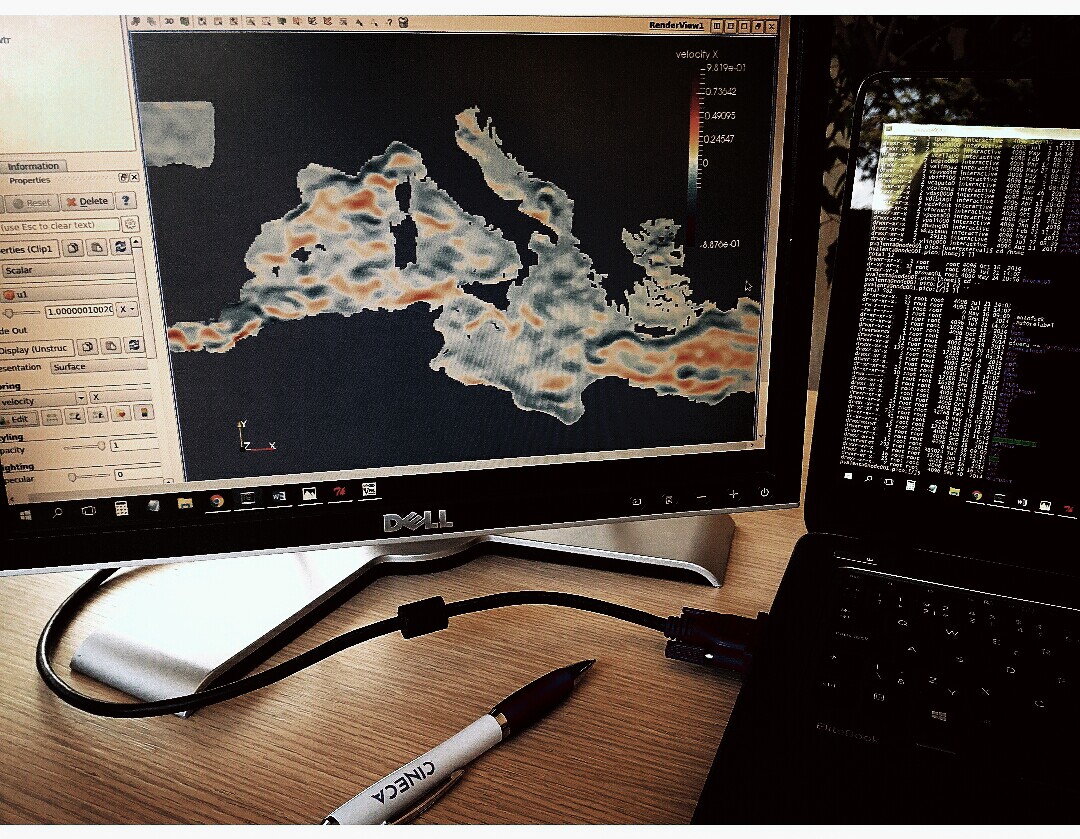
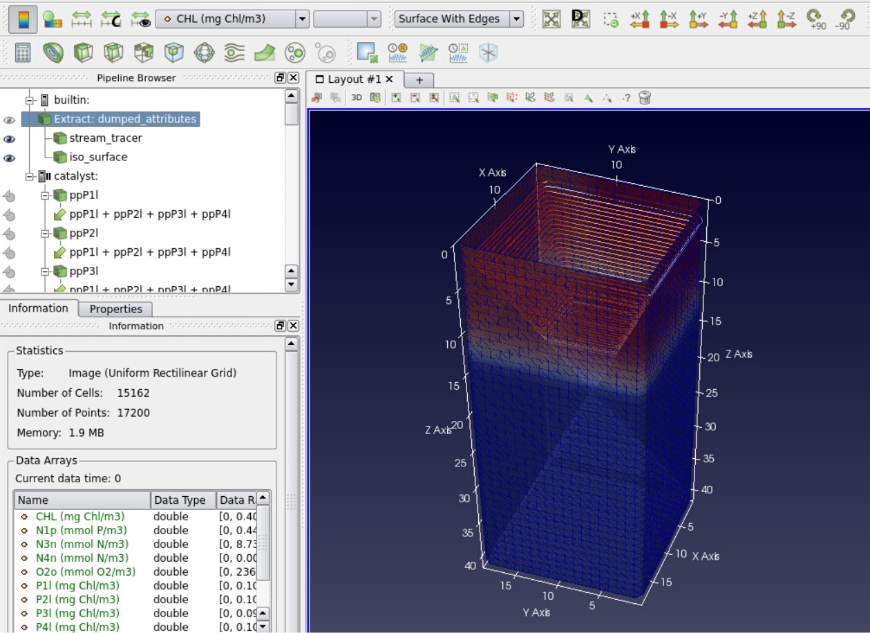
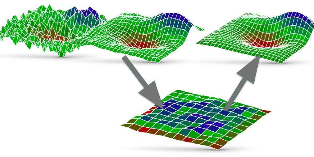
3D projection of the future workplace of a 2017 PRACE student at JSC
Project Mentor: Andreas Beckmann
Site Co-ordinator: Ivo Kabadshow
Learning Outcomes:
The student will familiarize himself with current state-of-the art GPUs (e.g. P100/R9 Fury) and accelerators (Intel Xeon Phi ‘Knights Landing’). He/she will learn how the GPU/accelerator functions on a low level and use this knowledge to optimize scientific software for CPUs/GPUs and accelerators in a unified code-base. He/she will use state-of-the art benchmarking tools to achieve optimal performance portability for the kernels and kernel drivers which are time-critical in the application.
Student Prerequisites (compulsory):
Prerequisites
- Programming knowledge for at least 5 years in C++
- Basic understanding of template metaprogramming
- “Extra-mile” mentality
Student Prerequisites (desirable):
- HIP/CUDA or general GPU knowledge desirable, but not required
- C++ template metaprogramming
- Interest in C++11/14/17 features
- Interest in low-level performance optimizations
- Ideally student of computer science, mathematics, but not required
- Basic knowledge on benchmarking, numerical methods
- Mild coffee addiction
- Basic knowledge of git, LaTeX, TikZ
Training Materials:
Just send an email … training material strongly depends on your personal level of knowledge. We can provide early access to the GPU cluster as well as technical reports from former students on the topic. If you feel unsure if you fulfill the requirements, but do like the project send an email to the mentor and ask for a small programming exercise.
Workplan:
Week – Work package
- Training and introduction to FMMs and hardware
- Benchmarking of kernel variants on the CPU/GPU/accelerator
- Initial port to HIP of one or two kernel variants
- Unifying the octree data structure for the CPU/GPU/accelerator
- Implementing multi-GPU support with HIP
- Optimization and benchmarking, documentation
- Optimization and benchmarking, documentation
- Generating of final performance results. Preparation of plots/figures. Submission of results.
Final Product Description:
The end product will be an extended FMM within HIP to supportCPUs/GPUs/accelerators. The benchmarking results, especially the gain in performance can be easily illustrated in appropriate figures, as is routinely done by PRACE and HPC vendors. Such plots could be used by PRACE.
Adapting the Project: Increasing the Difficulty:
The kernels are used differently in many placesin the code. For example it may or may not be required to use a certain implementation of the an FMM operator. A particularly able student may also port multiple kernels. Depending on the knowledge level, a larger number of access/storage strategies can be ported/extended or performance optimization within the HIP framework can be intensified.
Resources:
The student will have his own desk in an air-conditioned open-plan office (12 desks in total) or in a separate office (2-3 desks in total). He/she will get access (and computation time) on the required HPC hardware for the project and have his/her own workplace with fully equipped workstation for the time of the program. A range of performance and benchmarking tools are available on site and can be used within the project. No further resources are required. Hint: We do have experts on all advanced topics, e.g. C++11/14/17, CUDA in house. Hence, the student will be supported when battling with ‘bleeding-edge’ technology.
Organisation:
Jülich Supercomputing Centre, Forschungszentrum Jülich GmbH


 In my last blog post, I described general MapReduce paradigm which allows us to create big data processing systems in a fairly simple way. In this blog post, I will describe more in detail what I’m doing in my project, which big data framework I have chosen and what are the motivations for the project.


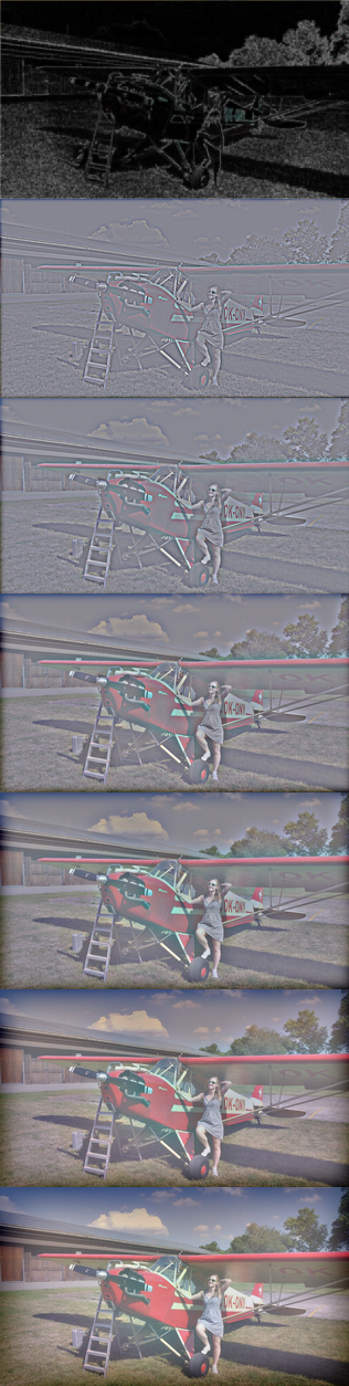
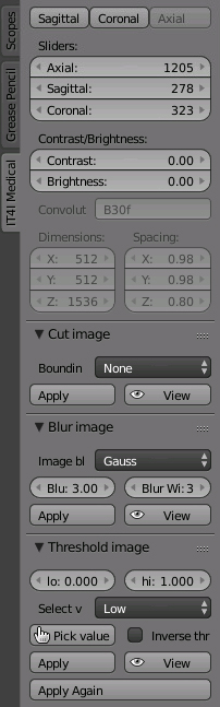 – The first three buttons determine from which axis will the scans be visible in our UV/Image Editor.
 – Applying the
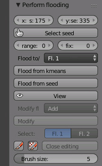

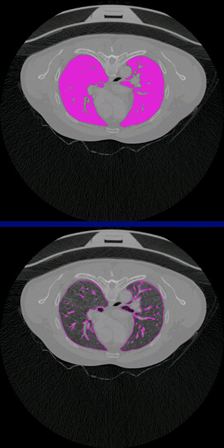
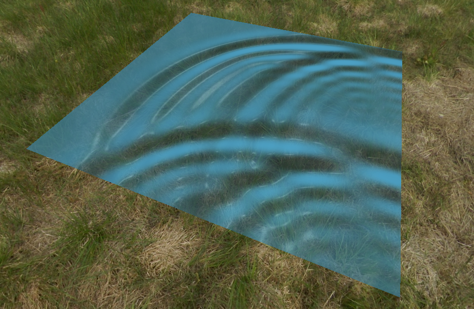
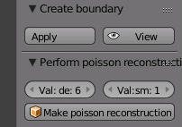 – The next step is to create boundaries, where it will detect where are the edges from the flooded surface and will draw them.
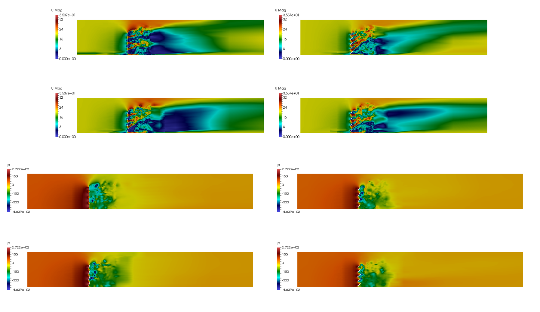
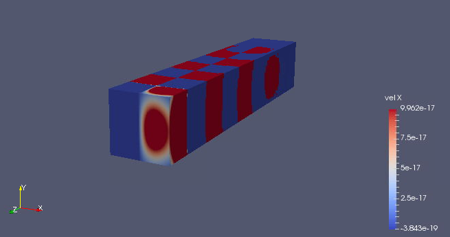
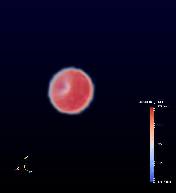
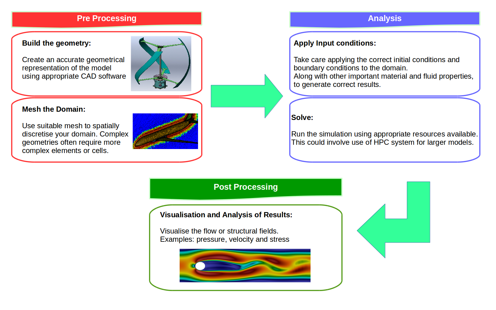 This project involved two pieces of software, OpenCASCADE, OpenFOAM and ParaView. As I mentioned in the previous blog, OpenCASCADE was used to build a series of geometric models, and subsequently OpenFOAM used to simulate the fluid motion before using paraview to look at the beautiful results. Given a picture paints a thousand words I’ll shut up and hopefully the image below will explain all the questions, you may have concerning this work flow, such as, “Wow Sam you seem like a really switched on guy with great hair and a lovely personality, please explain to me how this process is automated ?”


 Hi there!
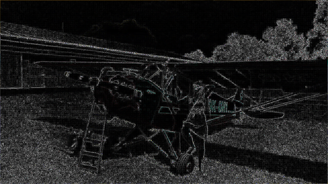


