Hi again!

Welcome to my second post, we are now in the fifth week of the program and everything is going so well for now. They always watch our progress and ready to solve any problems we have faced through.

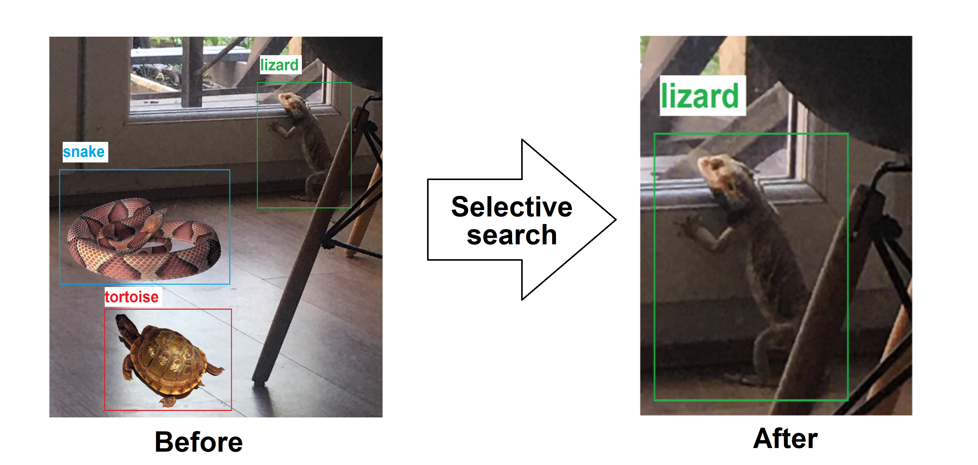
Coming to the project I am working on. Since the first week, we have been assigned to some tasks and tried to complete them in time duration given to us. In first couple weeks, we studied on Fault Tolerance Interface (FTI) library and did some implementations and tests to get familiar with it. We have also connected to the supercomputer and worked on it. We run our implemented applications on MareNostrum4 and made tests. Then, we discussed about process and decided to search and implement lossy compression and approximate computing techniques on checkpoints and compare them in next step. Firstly, we searched and prepared a presentation about topics, me on approximate computing and my project mate Thanos Kastoras on lossy compression. Next, in last and this weeks, we are working on implementing selected strategies to the library.

In my first post, which is here in case you haven’t read it yet, I have mentioned about the project generally. Now, let me tell a bit deeper.

FTI is application-level checkpointing which allows users to select datasets to protect for efficiency in case of space, time and energy. There are different checkpoint levels which are:

Level 1: Local checkpoint on the nodes. Fast and efficient against soft and transient errors.

Level 2: Local checkpoint on the nodes + copy to the neighbor node. Can tolerate any single node crash in the system.

Level 3: Local checkpoint on the nodes + copy to the neighbor node + RS encoding. Can tolerate correlated failures affecting multiple nodes.

Level 4: Flush of the checkpoints to the Parallel File System (PFS). Tolerates catastrophic failures such as power failures.

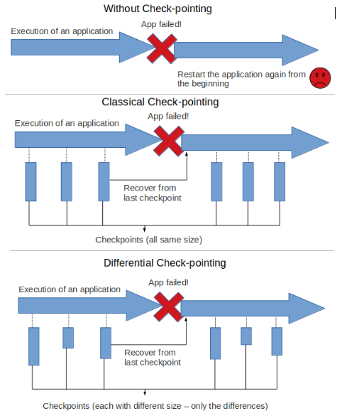
There is also one for differential checkpoint (dcp) which is L4-dcp. In differential checkpointing, only the differences from the previous one are held in checkpoints, thus decreasing the space usage. The difference between without checkpoint, classical checkpoint and differential checkpoint mechanisms can be seen in the simplified figure above.

Now, let me tell a bit about important functions which should be implemented in the application to provide FTI.

Firstly, at the beginning of the code FTI_Init(const char *configFile, MPI_Comm globalComm) function should be placed which initializes FTI context and prepares heads to wait for checkpoints. It takes two parameters which are FTI configuration file and main MPI communicator of the application.

Then, user should use FTI_Protect(int id, void *ptr, int32_t count, fti_id_t tid) to protect, store the data during a checkpoint and load during a recovery in case of a failure. It stores a pointer to a data structure, its size, its ID, its number of elements and the type of the elements.

There are two functions to provide checkpointing. When using FTI_Snapshot(), it makes a checkpoint by given time and also recovers data after a failure and it takes information about checkpoint level, interval etc. from configuration file. But when using FTI_Checkpoint(int id, int level), which level to use should be given as parameter. This function writes down the checkpoint data, creates the metadata and the post-processing work and as it is only for checkpointing before using this function, there are two functions to add for recovery part which are FTI_Status() that returns the current status of the recovery flag and FTI_Recover() function which loads the checkpoint data from the checkpoint file and updates some basic checkpoint information. These functions allow to see if there is a failure and start recovery if that is the case.

Finally, after all is done, FTI_Finalize() should be used to close FTI properly on the application processes.

These were some of important functions to implement FTI to an application and if you are seeking for more information, you can find it here.

Coming to the new functions we would add to the library:

Approximate computing promises high computational performance combined with low resource requirements like very low power and energy consumption. This goal is achieved by relaxing the strict requirements on accuracy and precision and allowing a deviating behavior from exact boolean specifications to a certain extent.

Checkpoints store a subset of the application’s state but sometimes reductions in checkpoint size are needed. Lossy compression can reduce checkpoint sizes significantly and it offers a potential to reduce computational cost in checkpoint restart technique.

That is all for now, I will tell more about precision based differential checkpointing which is the functionality I am trying to implement right now in my next post.

Hope you all a great day!

With a few weeks of progress into the program its high time to explain the project more in depth. The project title has given away a few key details – AI, linear algebra, and advanced algorithms – but how does it all fit together in the end, and how does it connect to the turtles from the title? Read on to find out.

Background

Assume that you are working on an advanced problem, perhaps the strength properties of a mechanical component which is in it self a part of an even larger problem, and you have through some amount of simplification and parameterization turned this into the problem of solving a large system of linear equations. Now, if this system is sufficiently large (our starting toy example is a sparse matrix in the range of 500k by 500k entries or 2.5e11 entries in total), even super computers have difficulties solving such systems in reasonable time. For this reason a number of algorithms have been developed to first approximate the solution as something known as a pseudo inverse or preconditioner, all in the name of just speeding up the solving step: We are specifically going to cover a Monte Carlo and stochastic gradient descent algorithm, but as the algorithms are not the focus of the project the specifics are left as an exercise.

The important detail is that the performance of these algorithms is entirely dependent on the choice of a couple of parameters, creating yet another layer of complexity. Our job is now to approximately find the best parameter choice for the approximate solution to an approximate system. This is where we start to approach the famous mythological concept of the world as resting on the back of a turtle, a turtle which as to not collapse must rest on another turtle, which of course must rest on another turtle and so on… It’s turtles (algorithms) all the way down, as commonly referred to.

Bayesian sampling based parameter search

We must stop this infinite chain of parameter search algorithms, and we do this with what is essentially a final through parameter search for all possible matrix configurations, finding the function of optimal parameters given a set of matrix features. This is something close to simply running a bunch of experiments to generate a lookup table, but as each evaluation takes so much time it is not possible to do this in an exhaustive way, leading to the need of a more in depth approach.

The solution is to build the model of the aforementioned function at the same time as you are doing the sampling. This allows you in each iterative step to find the preliminary optimal parameters, try sampling this configuration, and then refining the model specifically in that area updating it with the new data point, a technique called Bayesian sampling. The algorithm can also be seen as a form of reinforcement learning as it learns how to respond with an action (set of parameters) to an environment (matrix features), although I would argue this is more typically used in a more iterative process than the one studied here.

The solution however also introduces a set of sub-problems in what is hopefully the last complexity layer in the problem: We need to choose suitable matrix features which really are really closely correlated to the parameters, a suitable statistical model for regression, and a sampling strategy based on the statistic model for deciding on the next points to study. Finally we also need to do all of this in an efficient way to train the model with enough data points. These questions will all be revealed in the third blog post, so stay tuned!

Introduction

Hello everyone, welcome to my second blog post for the SoHPC 2021! I hope you are fine and enjoying the summer. It’s been a while since my first post so I will try to briefly inform you about what I have been working on for the past few weeks. For starters, I will introduce the concept of fault tolerance and the checkpoint-restart method. Then, I will explain lossy compression’s role in accelerating said method, which is the goal of my work. Enjoy!

The Need for Fault Tolerance

Current HPC platforms, consisting of thousands or even millions of processing cores, are incredibly complex. As a result, failures become inescapable. There are many types of failures depending on whether they affect one or several nodes, and whether they are caused by a software or a hardware issue, or by a third factor, but this digresses from this blog post’s scope. The mean time between failures (MTBF) of a large-scale HPC system is about a day. This means that approximately once a day the system faces a failure. Of course, all processes running during the failure will be killed and their data will be lost. This can be devastating on large-scale applications such as complex numerical simulations which may execute for days, weeks, or even months. Also, while HPC systems increase in scale (see exascale systems), MPBF decreases rapidly, creating many problems. Therefore, the development of Fault Tolerance mechanisms is necessary to be able to continue improving supercomputers’ performance.

This is a model of MTBF as a function of the number of nodes, with values from 1.000 to 10.000 nodes. The MTBF for one node is assumed to be 20 years, which means that a single node will fail once every 20 years. We can see that when approaching 10.000 nodes (a usual number for current HPC systems), the MTBF is less than 20 hours.

Checkpoint/Restart Method

Until this moment, the most common Fault Tolerance method is Checkpoint/Restart. Specifically, an application stores its progress (i.e. the important data) periodically during execution, so that it can restore said data when a failure occurs. Typically the data is stored at the parallel file system (PFS). The disadvantage of this method is that in large-scale applications there is an enormous number of data to be stored, and due to the file system’s bandwidth restrictions there is a high risk of creating a bottleneck and dramatically increase the processing time.

To fight such limitations, certain mechanisms have been developed in order to minimize the data which is written to the PFS, easing the file system’s work. Some of those mechanisms are listed below:

  • Multilevel checkpointing. This method uses different levels of checkpointing, exploiting the memory hierarchy. This way fewer checkpoints are stored at the PFS, while the others are stored locally on the nodes.
  • Differential checkpointing. This method instead of storing all the data in every checkpoint, changes only the parts of the already stored checkpoint which have been changed, decreasing the number of data that need to be written at the PFS.
  • Compressed checkpoints. This method compresses the checkpoints before storing them, again decreasing the number of the stored data. Usually lossless compression isn’t effective since it doesn’t perform a large reduction on the data size. Lossy compression, on the other hand, is very promissing and will be tested during our project.

FTI: Fault Tolerance Interface Library

Our project is based on FTI, a library made to implement four levels of Fault Tolerance, for C/C++ and FORTRAN applications. The first level stores each node’s data to local SSD’s. The second level uses adjacent checkpointing, namely pairing the nodes and storing a node’s data to both itself and its neighbor. This level reduces the possibility of losing the data since for that to happen two nodes of the same pair must die. The third level uses Reed-Solomon encoding, which makes sure that if we lose less than half of our nodes, doesn’t matter which, we can still restore our data. And the fourth and last level stores the data at the PFS. The goal of this implementation is that since the first three levels cover a large variety of failures, we can minimize the fourth-level checkpoints. Also, a differential checkpointing mechanism is implemented at the fourth level of FTI.

Lossy Compression’s Role

At Wikipedia, lossy compression is defined as the class of data encoding methods that uses inexact approximations and partial data discarding to represent the content. Namely, it’s a category of compression algorithms that do not store all the information of the compressed data, but a good approximation of it. The main advantage of lossy compression is that its error tolerance is a variable. Thus we can adjust the compression’s error tolerance to the accuracy of the application. While the error tolerance is lower than the application’s accuracy the application’s results remain correct. For higher error tolerances, we can achieve higher compression rates and increased efficiency. My job is to implement and test lossy compression in the FTI, using the lossy compression library zfp (by Peter Lindstrom, LLNL). After that, we will compare my results with the ones from my partner’s implementation of precision-based differential checkpointing, and gain conclusions.

A Quiz for You!

At the end of this blog post, I have a quiz to challenge you! Which of the aforementioned methods do you think is more efficient in decreasing the bottleneck of HPC applications and why? Multilevel checkpointing, Differential checkpointing, or Compressing the checkpoints? Provide your answers in the comments, and don’t forget to explain your thoughts! No answer is wrong, so don’t be afraid!

Talk to you soon!

Thanos

One step forward, two steps back. The reality in the world of programming: At one moment you are making progress, as easily and efficiently as standing your dominoes end-to-end and then you just nudge your first domino and hundreds of dominoes follow by themselves, and at another moment you try to fix a problem for three days, where you are not even sure if there is anything there to fix at all.

Me in the ‘Computerstraße’ (=computer street) in Vienna.

After the Training week I started with the system set ups on the UK national Supercomputer: ARCHER2, required for the MPAS atmosphere model runs. This has entailed, installing new modules, setting up directories for the libraries, like netCDF, or HDF5 for a parallel environment and preparing the Makefile for the MPAS installation. A lot of Errors came up, but I persevered on, and so I was able to go on to the next step: preparing MPAS for small runs, which means taking a small input mesh and a short simulation time. In principle there are two steps, that need to be done for this, the first, is to create from a mesh and from the input parameters, an initial condition file. And the second is, based on the initial file you can then run the simulation itself. To accomplish this well, and also with a view to future model runs, you try to write scripts for everything where it is possible. So of course, you need a job script, where you tell the cluster the details, like on how many nodes you like to run your simulation on, how and where the output should be stored, but especially also the run command itself. But it is also very useful to write a pre-processing, a run and a data visualization script, because it would be very time consuming to do this for every run ‘by hand’. In the previous week I was concentrated on the visualization script, which I decided to write in Python. Because on the one hand, Python is a widely used and easy to handle, and the other hand, it provides an interface to the netCDF library.

netCDF archieve structure. Credit: Hoyer, S. & Hamman, J.. (2017). xarray: N-D labeled Arrays and Datasets in Python. Journal of Open Research Software. 5. 10.5334/jors.148.  

This is important, because the output of the MPAS runs are netCDF files, where you have the 3d mesh coordinates, and physical relevant output parameters, like temperature at different pressures, wind velocity, vorticity etc. stored in n-dimensional arrays.

In my visualization script I load these Datasets, assign them to one dimensional Python arrays, and I am then able to plot them with matplotlib, like every other array. Of course, this is only one part of the story, the further step is connecting the visualisation script to the pre-processing and running script and that you enable the script in a way, that you just have to type in which parameters you want to have plotted and the rest is automated.

First visualisation attempt: spherical mpas mesh with 2562 grid cells, color-coded vorticity at 200 hPa.

Before we can visualize any data we have to produce a data set. We structure our test runs into small, medium and large ones. Where small/medium/large runs, are not only characterized by the mesh size of the model run, but also on simulation time and the core count we use for those runs. Additionally how different run parameters and some physical parameters influence the calculation time of our simulations will be investigated, as part of understanding the puzzle of MPAS and computational efficiency on ARCHER2.

Top left: me (Carla N. Schoder), Top right: Co-mentor Dr. Mario Antonioletti, Bottom left: Mentor Dr. Evgenij Belikov; Bottom right: Project partner Jonas Eschenfelder

Looking forward spending this summer together with Jonas Eschenfelder (check out also his Blog post on PRACE Summer of HPC website: ‘First steps with a big impact’), Dr. Evgenij Belikov and Dr. Mario Antonioletti on the Project: ‘Investigating Scalability and Performance of MPAS Atmosphere Model’ and report to you at least at the end of August about my experiences and results from this captivating project.

I am happy to meet you again in my second blog post. As I mentioned in my previous blog post, we implement the marching tetrahedra algorithm on the GPU to visualize the molecular surface.

First, the density at the grid points needs to be calculated. Since this process includes intensive computation, the process is done on the GPU.

How is the density calculated on a grid point?

The idea is to calculate the densities in each local grid and then aggregate them into the global grid. After obtaining the coordinates of the atoms in the PDB (protein data bank) file, the closest point for the global grid is calculated. Then atom density is calculated for each point in the local grid. One of the important points here is that the distance on the local grid needs to be converted to Bohr Radius. To compute an atom’s density at a grid point, Slater’s rule is applied. Slater Orbitals are an approximation of realistic orbitals. Since each atom has its own unique atomic number, the density of each atom must be calculated separately.

I mentioned the general idea to obtain densities on the global grid. Meanwhile, I mentioned some terms which are the local grid, the global grid and the densities of atoms. At this point, I am working on optimization by considering firstly the GPU architecture, paying attention to the per-grid floating-point instruction, per-grid memory access, branching diversity, the ratio of floating-point computation to global memory access metrics. While using these metrics, I use Nsight Compute as Profiling Tool. I am excited to share the results with you as soon as possible.

Thank you all of you for taking the time to read my blog. If you have any questions, I will be happy to answer them. You can write your ideas and questions in the comment. I hope to see you again in my next posts. 

Hi everyone! It’s Raska again here with a quick update on our Summer of HPC project. I gave little outline in my previous blog post (if you haven’t seen it, check it out here: (Machine) Learning How to Sea) and gave a quick intro on supercomputers. We’ve learned that they are essentially computers that work together to solve problems – here, we’ll discuss what specific problem we’re trying to tackle.

What’s the project about?

Me and Mario are trying to develop a computer program which uses artificial intelligence methods to automatically detect and classify reliefs in the sea, such as underwater mountains, trenches, canyons, and more. The method will be able to take in images of the deep sea and estimate what reliefs exist in the area.

All seabed maps in this article have been acquired by OGS (Instituto Oceanografia e Geofisica Sperimentale – Institute of Oceanography and Experimental Geophysics), under the framework of the MaGIC project (Marine Geohazards along the Italian Coasts) which was funded by DPC (Dipartimento della Protezione Civile – Department of Civil Protection)

Why are we doing the project?

A single patch of map from the MaGIC project with features manually marked [2]

In this project, we specifically focus on reliefs near coastal areas, because they are probably the most important part of the sea. Not only are they close to cities, coasts have a lot of marine biodiversity, and can their seabeds can contain important communications, power, and gas lines that these cities need. Coastal reliefs must be mapped out as it gives us an idea of what processes might happen under the sea, such as landslides and earthquakes. Knowledge of the likelihood of these processes can help us preempt and reduce their detrimental impact to such undersea assets, but most importantly to preserve the regional marine ecosystem.

Typically, these reliefs are classified and lineated manually. In other words, a team of marine geologists will look at a map of the sea and identify and mark out what reliefs exist in the region. This is a long task which requires the geologists to have a mutual understanding of all the relief characteristics. Because of this, we’re limited to how much information of the sea we can understand. However, an automated method can save time and also improve throughput; we’ll be able to classify more areas of the sea.

How does it work?

In our project, we use computer vision methods (a branch of artificial intelligence), which concerns how computer systems can interpret and understand images and videos. These methods can have a lot of daily uses; from recognising license plates of speeding cars to even facial detection for your holiday photos on Facebook! Much like teaching the names of objects to a human, we need to ‘teach’ the computer what each relief looks like, so in this case we need to use labeled ‘teaching material’ (in AI, we call this a training dataset).

A few years ago, a bunch of scientists involved in the Italian MaGIC project got together and went on huge boats equipped with measuring equipment to obtain relief maps of the Mediterranean sea. Their observations were then mapped and classified manually. Thanks to their effort, we now have labeled digital maps of the Italian coasts, which we now use as our training dataset as seen in image [2].

The Italian research vessel OGS Explora – one of the ships used to map out the coast [3]

The algorithm we are using is a type of Convolutional Neural Network (CNN) – if you are not familiar with these, all you need to know is that they’re an artificial intelligence algorithm inspired from how humans perceive sight. CNNs are common in image and video recognition; here, we use them to recognise ‘images’ of the seabed. Bear in mind, these ‘images’ aren’t just pictures of the sea; these are mappings of the measurements done by the scientists in the MaGIC project.

We ‘cut’ these images into small parcels that are each labelled as one specific type, in a process called Selective Search. Again, same like teaching to a human, if we wanted to teach someone how to differentiate between lizards and other reptiles, we’d ideally like to show it a good image of what it looked like, preferably without any other reptiles around it, to avoid confusion.

Selective search on an image of reptiles to focus on a lizard [4]

We then feed these labelled images into our algorithm so that it can update itself until it meets a satisfactory accuracy level – this is called training a model. The dataset we generated is massive, and our CNN is also heavy to calculate, therefore we need a lot of computing power. This is why we are using Marconi100, the main supercomputer at CINECA. At the moment, it’s the 14th most powerful computer in the world!

Our buddy Marconi100 has helped with generating the dataset from the labeled maps and setting up preliminary models. This third member of our team is powerful enough (and possibly much smarter than me and Mario combined) to run our program, as it uses a method called parallel computing – this means that certain sections of the program is run together by different components of the computer, making it much quicker than running using one device.

How is the project going?

Some snapshots of training data for our neural network taken from a map of the sea [5]

Pretty good, I think! We’ve had a few hiccups dealing with converting the data from GIS files (Geographic Information Systems – a type of software used by geologists to analyse map data) into a good format for our model, but we’ve now trained some models with varying accuracy, using a single patch of map from the MaGIC project. We still think there is more we can do to improve it until we’re certain we want to deploy our model to predict larger areas, such as the entire MaGIC repository.

A little question before we go:

[5]

Last time, we discussed what supercomputers can be used for – I was really glad to see your enthusiasm for supercomputing. Here, we’ve learned how we can use artificial intelligence, specifically computer vision, to detect undersea reliefs. Besides this, AI methods come in a lot of forms for different functions. So, my questions are:

What do you think AI can do?

What comes into mind when you hear the phrase Artificial Intelligence?

Leave your answers in the comment section below!

Image references

[1] Coastal reliefs – Encyclopaedia Brittanica

[2] Patch of Calabrian coast – Istituto Nazionale di Oceanografia e di Geofisica Sperimentale

[3] OGS Explora – Istituto Nazionale di Oceanografia e di Geofisica Sperimentale https://www.inogs.it/en/content/research-vessel-ogs-explora

[4] Selective search – Authors own image, also using images from https://pngimg.com/image/4065 and https://www.schoolphotoproject.com/animals/tortoise-photo5.html

[5] Free question stock photo – FreeImages https://www.freeimages.com/photo/question-1239547

(Above is an example of a molecular dynamics simulation, where Nitrogen is the diatomic system we’re particularly interested in).

This week marks the halfway point of PRACE Summer of HPC, and we have learnt so much since starting. We have made really good progress with our project, thanks to the support from our mentors. Read below to see what we’ve been up to!

What does the project involve?

So, what does “Molecular Dynamics on Quantum Computers” actually mean?  In a nutshell, we are finding the ground state energy of a diatomic system by implementing a Variational Quantum Eigensolver (VQE). This requires finding the minimum eigenvalues for the Hamiltonian operator, in the Schrodinger equation, using quantum algorithms and classical optimisation techniques to fine tune these estimates.

This is a highly valued application of quantum computing, as finding the ground state of molecules allows us to understand reaction rates better, and thus provides scope for drug discovery. It means that we can make predictions in quantum chemistry, without physically going into the lab and testing out different reactions. However, these simulations become increasingly more difficult as the molecules get larger and more complex. Right now, we are at the infancy stage of quantum computing – imagine the ground-breaking discoveries we can make when its full potential is unlocked!

What have we done so far?

The project is split into two main parts: VQE, and the Quasi-classical trajectories method (QCT). The aim is to join these two parts into one molecular dynamics simulation to get an accurate solution to the Hamiltonian.

The Hamiltonian acts on a wave function, and can be difficult to solve as it requires excessive computation. However, using the Born-Oppenheimer approximation, we can split the Hamiltonian into two parts (the kinetic term and the electronic Hamiltonian) and solve them separately. The separation is done based on the assumption that the nuclei is much heavier in mass than electrons, and therefore can be assumed stationary.

This week we built and finalised our VQE in Qiskit to simulate a hydrogen molecule. We initially ran the VQE on a state vector simulator, as demonstrated in IBM’s Qiskit tutorial after which, we tested the VQE on both a qasm simulator and real quantum computer. We also tested these methods using different optimisation techniques, namely COYBLA and SLSQP. The purpose of this was to compare the results against each other to find the optimum simulator and optimiser, whilst also creating artificial noise to investigate its effect on quantum estimations. One of the key challenges facing parameter optimisation is the noise associated with quantum hardware; its presence suggests that the energy calculation may not be the true objective function. Therefore, in the next few weeks, we will explore noise-mitigation techniques.

Our results above show that the state vector simulator emulates ideal execution, with the exact energy and VQE energy matching up nicely. On the other hand, the qasm simulator, which is the main Qiskit Aer backend, simulates the VQE on a real device, and includes noise models based on actual quantum hardware.

What are our targets for next week?

Next week, we will focus more on dynamics, looking at the equation of motion used for semi-classical approximations and the Born-Oppenheimer approximation, to ultimately perform calculations on the vibrations of the hydrogen molecule. However, we will first need to define a function for the numerical evaluation of the energy gradient in order to do this.

Stay tuned to hear more about our progress!

Hello! Over half of the Summer of HPC programme is already in the past so I figured it was about time to update my blog accordingly. Over the past month, we have had the chance to meet a lot of different people from the Computational Earth Science department at the Supercomputing Center in Barcelona, and more specifically the post-processing team. In addition to this, we of course gotten familiar with the Interpolation Tool and started working on the bugs and features we should try to fix and implement.

What is this Interpolation Tool?

The Interpolation Tool (Abbreviated ‘it’, exactly like Stephen King’s 1986 horror novel) is, as stated in its name, a tool that performs interpolation on a given set of points. Often, when performing measurements or forecasts as in our case, the resulting data comes in a form that does not exactly suit your needs. There could for instance not be a station at the point you need data about. In this case, one should use the given observations/forecasts in order to make an educated “guess” about the data lying in between the existing points. Depending on the interpolation method, this requires a lot of computational power even for small datasets, so there is definitely a need for HPC when dealing with large data.

What am I doing?

This tool has been in development for already a few years, but still presents some bugs misses some features. That is where we step in! Over the course of the past month, I have been transforming the standalone tool into a Python package, integrated pointwise interpolation and am now working on solving a known “freezing bug” occurring under specific configurations. Now that I have a deeper understanding of how the package is working I feel like I can work more efficiently and achieve the wished goals. Once these tasks are finalized, I hope to still have time to implement another type of grid the tool can interpolate to.

Although we are not in Barcelona I do still find a way to enjoy the nice Dutch weather, and hope you do so as well! If you have any questions please ask them in the comment section or feel free to reach out to me on LinkedIn.

My job is to create a virtual replica of the Marconi 100 supercomputer in which you can visualise data such as the status and temperature of each node. To do this, we first need to know the technical specifications of this machine.

Architecture of Marconi 100

Marconi 100 is a supercomputer created by IBM and launched in 2020. It is composed of 55 racks, 49 used for computing nodes. Each rack has 20 nodes, named using the rack number followed by the node number. For example, node 5 in rack 210 is named r210n05. In turn, each node is composed of 2 CPUs of 16 cores each and 4 GPUs. As a curiosity, with its 32 Pflop/s, it was the ninth largest supercomputer in the world in 2020 and uses the Red Hat Linux distribution as its operating system.

Data to be displayed

The data is contained in an ExamonDB database. Since it is a very large amount of data and we want to facilitate its management, it is stored in a different file for each node, that means 980 files.

The database has information since the supercomputer was started. Data such as the temperatures of both the CPU cores and the GPUs. The power, voltage and memory consumed by each CPU. And one of the most important data for us is the status, which indicates whether the node is working properly or has a problem. A value of 0 means that there are no problems and any other value means that there is a problem.

Creating the 3D visualisation

To create this visualisation we used the VTK (Visualization Toolkit) package for Python and Pandas to handle the data in table form. The CINEMA visualisation team provided me with a 3D model of Marconi 100 which I exported in STL format, as it is very easy to load with VTK’s vtkSTLReader class. (Provigil)

The VTK visualisation pipeline consists of the following parts: Sources, used to read raw data. Filters can then be used to modify, transform and simplify that data. Mappers are responsible for creating tangible objects with the data. And at the end of this pipeline are the Actors, which are responsible for encapsulating these objects in a common interface that has many freely modifiable properties. These Actors are the ones that are passed to our renderer to show them in the scene. In addition to all this, other much more specialised classes can be created that allow us to develop a more interactive environment, among other things. (messinascatering) In my case, I have used this to create keyboard shortcuts that I use to move around the time axis when displaying data.

VTK Pipeline

Using all this I have created a first 3D visualisation version of Marconi 100. In this version, I show the status of each node with a coloured plane (green if it is working properly and red otherwise). A text with the consumed power is also shown. And for quicker identification of each node, there is a text with the rack number above it. You can see it in the video below.


The next step is to improve the graphics by adding textures and new data such as core temperatures, where they could be interpolated with a temperature point cloud. In addition, data loading can be improved by parallelising the process.

Hello ! 
Welcome to my blog post #2 where we get deep into the MEEP! If you have not yet read #1 you can do so here . In this post , I will give more comprehensive outlook to the project and talk about my progress as well.

The Memory Hierarchy

Before delving into the nitty – gritties of the project, it is important to understand what the memory hierarchy is and why it is a fundamental factor that determines the performance of any computing system.

Imagine there’s a large store in your city (This is obviously before the times of online shopping). İt is well stocked and has got everything you can think of , from a lawnmower to kitchen napkins. But there’s a catch. Shopping in this store takes quite some time because :

  1. Since it has so much stuff, you have to go through so many aisles to get to what you need.
  2. The store is located further away from your home .

Time is money, so your city’s municipality decides to build a smaller supermarket near your neighborhood. It is not as equipped as the mega store , but it has most of the stuff that you need frequently. Furthermore, if you ever needed anything that is only in the larger store , it could be fetched and brought to the small supermarket. Pretty cool, right?

This is basically how the memory hierarchy operates. We have smaller, faster memory levels placed closer to the CPU (Central Processing Unit) and they contain only the data and code we need at the moment, hence faster speed in processing.

Need for Speed

This project proposes various placement and management policies that optimize the movement of data and instructions through the memory hierarchy. These novel policies would have to be tested and experimented upon before casting them onto silicon and MEEP offers an excellent platform to do this.

MEEP (MareNostrum Experimental Exascale Platform), is an FPGA (Field Programmable Gate Array) – based platform that enables us to evaluate new architectural ideas at speed and scale level and also enables software readiness for new hardware. It would be easier to think of MEEP as a foundational prototype that can be used to test the viability of a certain framework or architecture. One of the unique features of MEEP is a self-hosted accelerator. This means that data for the calculations can reside in the accelerator memory and does not have to be copied to/from the host CPU. This accelerator is part of the chiplet architecture called the ACME (Accelerated compute and Memory Engine). A key differentiator of ACME is that it employs a decoupled architecture in which the memory operations are separated from the computation. While dense HPC workloads are compute-bound in which the accelerator tiles represent the bottleneck, sparse workloads are memory-bound as the vector elements need to be gathered/scattered using multiple memory requests.

Coyote Simulator

The cherry-on-top to this accelerator of the future is the Coyote simulator that is responsible for its performance modelling and analysis. My role in this project is centered around this simulator, the MCPU simulation specifically. Coyote is founded on existing simulators (Spike and Sparta) and is being improved by catering for their shortcomings,especially in the HPC domain in which the number of resources to be simulated is high, hence making it a powerful modelling tool. The name “Coyote” was adapted from the Looney Tunes cartoon series “Wile E. Coyote and the Road Runner”.

These past two weeks, I was busy setting up the simulator repository and dependencies in my PC and working on scheduling policies of load and store instructions within the MCPU . The latter is still a work in progress and I plan to expound on it in my next blog post.

Emulation … Simulation … what’s the difference?

Simulation involves creating an environment that mimics the behavior of the actual environment and is usually, only software oriented. Emulation, on the other hand involves duplicating the actual environment both in the hardware and software spectrum. Below is an illustration of how the MEEP project implements both emulation and simulation.

And that’s it for blog post #2. This was a long one so congrats if you made it this far. I hope you have learnt something new or gained a clearer perspective of our project. I’d be happy to answer any questions you may have about the project so feel free to comment below.

Blog post #3 coming soon!

Hello again!

With the third week of work in the books, it’s high time for another update here. We’ve been busy getting everything set up on ARCHER2 to be ready to run proper simulations and get into the performance measurement of the MPAS atmosphere model.

After some technical issues with downloading and compiling MPAS during the first week, we set our eyes on writing scripts to help automate future runs. As we intend on simulating a wide variety of scenarios using different parameters such as mesh size, model run time and number of nodes used, not having to manually change these for each run will save a lot of time in the future.

Figure 1: An idealized baroclinic wave simulated for 150 hours propagating through the world’s atmosphere

Last week we were finally were able to start running the first simulations. This wasn’t a real test scenario yet but a simple idealized case. Figure 1 shows the result of a Jablonowski & Williamson baroclinic wave modelled for 150 hours (just over 6 days) propagating across the Earth. This is a very simple test often used to see whether an atmospheric model fundamentally works. It models a single pressure wave propagating zonally across the Earth.

Figure 2: Plot of average run time by number of cores for a 150-hour simulation of a JW baroclinic wave.

While not very exciting to look at, these kinds of tests help us to see whether MPAS is working properly and also gives us an important insight into how we can best design our upcoming experiments to make the best use of our time and computing budget. It also gives us a first look at the performance of the MPAS atmosphere model. As seen in the Figure, the average run time dropped from 1 to 3 cores, showing better performance with more computing power, but increased again when 4 cores were being used. This is most likely due to any performance gain by further parallelization of the model being diminished by more time spent in communication between the tasks. These are the kind of insights that we hope to find later in our performance analysis, but on a much bigger scale, and will investigate using profiling tools to pinpoint where performance is lost.

With the experiences gained from the last few weeks, we are now ready to start the proper performance analysis of MPAS, next up is debugging some of the automation scripts and running small scale simulations for our first real scenario. So, stay tuned for more updates!

Hi everyone, my name is Rajani Kumar Pradhan, and I am from India (Andhra Pradesh). Currently, I am pursuing my PhD in the Department of Water Resource and Environmental Modelling, at the Czech University of Life Sciences Prague. My research interest is centred around satellite precipitation, climate change, hydroclimatic variability and the global water cycle.

Before starting my PhD, I have worked as a ‘Junior Research Fellow’ at Banaras Hindu University, India. Even before that, I have completed my master’s in environmental science, from the Central University of Rajasthan, India. Although I have some general idea about High-performance Computing and Big data, however, the real encounter started when I faced some huge datasets. This is the moment when I realized the importance of HPC in data analysis and thanks to my supervisor Yannis Markonis, who introduced and shared the information regarding the PRACE Summer of HPC 2021.

The journey has been started with a one-week training programme from introducing the basics of HPC to some advanced topics. It is unfortunate that we cannot meet or attend in person considering the pandemic, however, the online meeting with zoom also has some unique experience. During the training week, I have introduced to several new terms like MapReduce, OpenMP, MPI and most of them I never heard before. To bring some more fun into the programme they have also scheduled some hands-on exercises, following the lectures.

And coming to our main project, the training programmes offered several excellent diverge projects. Among them, I have selected project number 2133 The convergence of HPC and Big data/HDPA, which I find more interesting and very relevant to my needs. The main motivation behind the project is how to tackle the challenges in the convergence of Big data analysis with HPC.

During the following week, I have started our main projects with Giovana Roda, and college Pedro Hernandez Gelado. We have started with another training week and some basic introduction about Hadoop, HDFS, and Spark. At the same time, we have some exercises to practice on the Vienna Scientific Cluster(VSC-4). Initially, we have started with the Little Big Data (LBD) and later we have worked on the VSC-4. In the upcoming weeks, we will work on some case study datasets on the cluster and cannot be more excited about it! Stay tuned, will come with new updates in the upcoming weeks.

Until that bye..!

In my last blog post, I presented the Boltzmann-Nordheim equation and that Supercomputer can help us to solve this equation. This time, we have a look at the Supercomputer itself and how we can use it.

Why do we need Supercomputers?

Before having a look at supercomputers, we might ask ourselves, for what kind of problems do we need them for? One major application of supercomputers is simulations. A current example for simulations is the COVID-19 Pandemic, where PRACE supports projects focussing on different aspects of the crises, as simulations of the spread of the disease or research to understand the virus itself.
Another example is the weather forecast, where supercomputers use the current weather to predict the upcoming weather. You will find many more examples, where supercomputers play an important role.

Could my computer solve these problems?

For some of these problems, your personal computer might be able to compute a solution, but not to the precision that would satisfy the scientific needs and standards. Furthermore, your computer would just take too much time to finish the task. In the last weeks, I tried to run the code that simulates the Boltzmann-Nordheim equation on my computer at home – after an hour of waiting for a response, I just stopped the computation. Luckily, my supervisors gave me access to a more powerful computer, where I did not have to wait hours to get a result.

But what makes it faster?

It is not just, that supercomputers have a faster CPU or a bigger RAM than your PC (the Fugaku, currently the fastest Supercomputer has 64PB RAM!). Their major strength is, that they have more CPUs than your PC. This way, you can more think about multiple Computers working together rather than a single big machine! In the video below we can see how we can benefit from having multiple CPUs.

The “PRACE” mesh was generated via png2mesh, a c++-library by Johannes Holke to produce meshes given a .png files. The backbone of the project is t8code, a library to manage the adaptive mesh refinement in your project.

And how does that relate to your project?

In the video of the last post, I showed you, that I am focussing on a part of the equation, that describes the collision of the particles. My supervisor, Alexandre Mouton has developed a method that can further subdivide the collision term into pieces, such that they can be computed in parallel. My task is to get a good understanding of this method and to add it to the current state of the code.
In the last weeks, I had a look at his code and installed it onto my computer. Before editing the code, I need to understand it. With thousands of lines of codes, it was not easy to get into it. Luckily, I do not have to read and understand all of them as I do not have to adapt the whole project. Recently I started to implement the new method and planned what parts of the method I will focus on in the next weeks.
For now, I will head back to coding, but keep you up to date on every progress with the upcoming posts.

Hi again! It’s been a while now, and I have finally gotten to begin working at the Barcelona Supercomputing Centre, helping improve their interpolation tool for atmospheric models! I have gotten to meet the team at the CES department (Computational Earth Sciences), and it has been a blast so far. The interpolation tool is used for regridding atmospheric models in post-processing, outputting the model data in various different ways depending on how it’s needed. This way, we can provide excellent flexibility with the tool. What I am doing now and will continue to do in the next few weeks is trying to improve the performance and scalability of the interpolation tool using HPC techniques and any other innovations that I can come up with.

What is the interpolation tool?

Interpolation is a very powerful mathematical method where we can take a datapoint or datapoints in a time-space domain with some measured variable. Then, we use a combination of these datapoints’ measured variables and positional values in space and time to infer the variable at some nearby, unmeasured point. This enables us to flexibly reconfigure datasets and potentially even increase their resolution! Naturally, one is dealing with large, multi-dimensional arrays when dealing with these types of problems which is where HPC can become incredibly powerful.

Currently, the interpolation tool at BSC interpolates atmospheric variables both vertically and horizontally, vertically using the spline interpolation method, and horizontally using the interpolation package provided by pyproj in Python. The vertical interpolation can be easily parallelised because of its separate layers using MPI, however this is not so simple for horizontal interpolation, which is currently only parallelised using one node.

So what am I doing?

Right now, the horizontal interpolation is carried out before vertical interpolation. What I plan to do is reverse this order. By doing so the horizontal interpolation processes may be able to take advantage of the parallelised vertical processes, and by doing so essentially become parallelise itself and much less computationally demanding. I have been working on this with my mentors and colleagues at BSC, and soon hope to be able to implement my changes into their system. Afterwards I plan to move on to a second task, improving the scalability and performance of the tool’s horizontal interpolation. Currently, this is done using a technique known as pickling, python objects are serialised and stored for later reopening. By doing this, the local memory is freed up for other processes, greatly improving performance. I hope to further optimise this process and see if there are any additional improvements or ideas I can introduce into to tool. I’m super excited to see what I can come up with!

CerModern

Hello everyone! My name is Ceren. I am a final year student of Mechanical Engineering at Gazi University. I was studying industrial engineering in the first two years of university, but when I realized that this was not my dream, I transferred to the mechanical engineering department.

I love watching anime, playing basketball with my friends, hiking in nature, and listening to music. You can share your playlists with me. We can talk about music.

I met HPC at EuroCC@ Turkey High-Performance Computing Winter School. I realized that HPC is necessary for the job I want to do. After researching further, I saw the PRACE Summer Of HPC program and decided to apply. There were projects with incredible content, but I applied for the project coded 2128 in line with both my competence and my field of interest.

While preparing a report for the Jet Engine Design competition with my friends, I saw the acceptance email. I excitedly verified the content of the e-mail to all my friends. I really felt very happy.

As a participant of SoHPC 2021, I will be working with my project partner Bartu Yaman on the topic of S-gear geometry generation and optimization algorithm based on transient finite element mechanical/contact analysis.

In the first week of the program, they gave us training on the program process and on Python, Cython, OpenMP, MPI. Our instructors were really interested in teaching and answering questions.

What is the purpose of the project with code #2128?

The project has two main objectives :

  • Optimization procedure, based on transient finite element (FE) mechanical analyses of the gear meshing process, will also have to be developed and implemented using open source and/or commercial FE software inside an available HPC cluster.
  • Developing a custom algorithm that will enable the generation of both spur and helical type 3D gear geometries in CAD format.

This internship program is very important for me. Thanks to the internship program, I will learn new information, improve myself in engineering and find an answer to the question of which master’s degree program I should choose.

I will talk a lot about the project content in my next blog posts. You can easily contact me. I wish you all a peaceful day.

Hello everyone! I am Şahin Can Alpaslan from Turkey. Graduated from University of Kocaeli Chemistry department. I will be working project 2126 Benchmarking Scientific Software for Computational Chemistry in the Dutch National Supercomputer at SurfSara BV. The goal of this project is to get acquainted with different relevant software for scientific simulations and be able to analyse and describe the performance of the most relevant applications that are currently run by researchers in the field.

This image has an empty alt attribute; its file name is 20210712_215048.jpg
Kocaeli Archeology Museum

Contrary to the general story, I was only interested in video games in my childhood, not programming. It didn’t take long for me to meet computational chemistry after I entered the chemistry department because I became interested in software. As I started to discover chemistry, I started my computer-aided chemistry research, thinking how I can speed it up and here I am!

I met HPC systems with Introduction to supercomputer training. Then I followed the trainings, met the people working on this subject and applied to PRACE Summer of HPC program.

What am I interested in besides HPC system and chemistry?

This image has an empty alt attribute; its file name is 20210712_215038.jpg
Autonomous Car Training
  • Flying things
  • R/C
  • Anime
  • Researching what interest me

Feel free to follow the links below to know more about me and my work:

https://www.linkedin.com/in/%C5%9Fahin-can-alpaslan-331865131

https://twitter.com/sahincanalpasla?s=09

Thanks for getting to this point, I will be glad if you follow my blog. Do not hesitate to ask questions!

See you next post, be safe!

Introduction

Hello, my name is Martin Stodůlka and I will use this blog post as a way to introduce myself. I am 25 years old and I was born and still live in town called Brno located in Czech Republic. I have earned my Master’s degree (Ing. title in my country) this year with specialization in HPC. I’ve graduated from both Bachelors and Masters on Brno University of Technology – Faculty of Information Technology.

Even prior to university I attended a grammar school Vídeňská which specialized in programming where I had my first experiences with programming. Outside of school ever since I was 18 years old I worked part time during summer holidays in a company Tescan which specializes in manufacturing and developing electron microscopes and the software that operates said microscopes. I mostly developed tools for processing large data and worked on some image processing methods as well.

Outside of programming I am just an average guy who likes: tourism, sight seeing, PC building and gaming. I used to go fishing and collect minerals when I was younger. As of late I have been thinking about getting into airsoft to get some more physical exercise and keep in touch with my childhood friends.

Why have I chosen SoHPC and what do I expect from it?

I have chosen Summer of HPC to test and expand my skills learned at my university. I am also hoping to explore new environment, people and perhaps opportunities. I have learned about Summer of HPC during one of lectures about HPC, where previous absolvents shared their experiences with Summer of HPC.

The project I am working on

I have been assigned to a project called Designing Scientific Applications on GPUs with my colleague Theodoros and my mentor for this project is Dr. Ezhilmathi Krishnasamy. For the rest of the summer I will be working on optimizing application for large scale topology optimization called TopOpt which uses library PETSc which is used for highly parallel scientific applications modeled by partial differential equations. My goal is to locate slow parts of code in TopOpt and speed them up using CUDA/GPUs and replace CPU PETSc code with GPU variant.

Solution produced by TopOpt

Hello and welcome! I’m Cormac McKinstry, and I am delighted to be part of PRACE’s Summer of HPC 2021.

How did I get here?

I’m coming to you from my family home in Galway, on the west coast of Ireland. While the opportunity to work in Nice is sorely missed, it hasn’t been a bad spot at all to sit out a pandemic. I recently graduated from by Bachelors in Theoretical Physics at Trinity College, Dublin. While physics may have been a major part of my degree, computer science and the limits of computing technology are something I’ve held an interest in for a long time, and I’ve recently been accepted to do a Masters in Quantum Science and Technology, focusing on Quantum Computing, starting this September back at Trinity in Dublin.

This isn’t my first experience working with High-Performance Computing. Last year, I had the wonderful opportunity to work with ICHEC, the Irish Centre for High End Computing. There I worked on simulations of Quantum Computing algorithms, learning how to program for quantum computers. I worked on simulations of quantum chemistry, using QC to calculate the energy levels of molecules. This got me started working with both Quantum Computing and HPC.

What am I doing here?

For the next couple months, I have the privilege of working with Daniel Pino Muños from Maison de la Simulation (MdlS) in Nice France. In collaboration with my partner Mukund, we will be developing a thermal model of Regolith in space. The interest in this is driven by the OSIRIS-REx space exploration mission, which you may have heard about when it traveled to the asteroid Bennu and landed in 2018. From it we learnt that the surface of Bennu is covered in a surface of loose, small, unconsolidated stones called regolith. The 2018 landing recovered a sample of the sample that will arrive on Earth in 2023.

Model of heat transfer in regolith

We want to understand the thermal properties of this regolith. To do this, we will be creating a parallel radiative heat exchange solver, simulating the thermodynamics of the regolith under various circumstances in order to understand what we’ll see from measurements. This is no easy task, but it’s one I’m excited to get going with.

Image Source: Ryan, Andrew & Pino, Daniel & Bernacki, Marc & Delbo, Marco. (2020). Full‐Field Modeling of Heat Transfer in Asteroid Regolith: Radiative Thermal Conductivity of Polydisperse Particulates. The Journal of Geophysical Research Planets. e2019JE006100. 10.1029/2019JE006100.

This is Paolo Scuderi from Italy. Well guys, I am 25 years old and actually I am not a student anymore. I have just graduated from Politecnico di Torino a few days ago at DIMEAS Department. However, let me introduce who I am and how I was put in contact with PRACE.

Something about me

I am an Aerospace Engineer, graduated cum laude on the 14th July 2021. I spent the last year developing my Master’s Thesis in collaboration with The von Karman Institute for Fluid Dynamics, in Belgium. Unfortunately, due to the strange and hard Covid period, I was not able to reach the Institute and spend some days on-site. I worked online. At the beginning of that experience, I was sad. Of course, traveling and working on the project that you love is the happiest combination that every student-researchers would like to join. Anyway, having spent many hours in front of my PC, I joined CINECA Academy. With their continuous support, I met PRACE and I discovered a new passion regarding High-Performance Computing! Which is the best combination? I studied Aerospace Engineering and I specialized in Fluid Dynamics. As you know, I think, the Navier-Stokes equations are not analytically solved. Hence, only two different approaches are possible: the experimental one and the numerical one. The former is very expensive and not usable during a period like this. In this context, my Master’s Thesis has been associated with the numerical idea. In addition, as a consequence of the high computational cost of these simulations, the HPC systems have a lot of applications in the fluid dynamic world. For these reasons, when PRACE was presented to me, I felt incredibly motivated and I started to find some projects related to my field of studies. I found Summer of HPC, an amazing and interesting project which aim is to provide good knowledge of the usage of HPC systems around Europe to all the students. What’s better than this? Well, there was only one problem: finding a project related to Fluid Dynamics. Fortunately, the idea comes from the University of Luxembourg, where I am currently working.

Aerodynamic project at University of Luxemburg

My project aims to study the behavior of the external flow over the DrivAer car model developed at TU Munich. There are several configurations based on the shape of the geometry of the top, the underbody geometry, the mirror configurations, etc. … Cars, from an aerodynamic point of view, are blunt bodies. The typical two elementary contributions to the forces are pressures and stresses. When we are talking about blunt-body the first one is bigger than the second one. Hence, this is the case of DrivAer problem. For these bodies, a big wake is present in the region behind the car. The presence of the wake is associated with the lack of momentum, which is again related to the component of the total aerodynamic force projected in the parallel direction of the infinity flow: the drag. This is only one of the contributions to the total drag of the cars. Indeed, for instance, also the wheels and the underbody region contribute to it. As a consequence, to make the cars move, they need to develop a motor force such that it can win the negative contributions related to drag. In this context, the cars use combustible fossils to develop this force. The chemical energy provided by the reactions is transformed into mechanical energy thanks to the engine. As a result, a large amount of waste is released into the environment. One of the most important aims of car aerodynamic studies is to find the mechanism to reduce the drag, to finally reduce carbon dioxide and the NOx in the Earth’s atmosphere. These concepts are not valid for motorsport cars, where the main goal is to develop an aerodynamic body to reach the highest velocity possible. Indeed, drag is the most important aerodynamic force when the car speed is very high. Therefore, talking about urban cars, drag is more relevant in the motorway instead of in the normal urban city. However, the aerodynamic studies were not important until the energetic crisis of ’70. Nowadays, the aerodynamics of urban cars is important to save our environment. I am studying all these aspects in my project!

Something about you

And now, some questions for you. Are you ready? Feel free to answer and contact me, there are no wrong answers. We’re all here to learn something new!

Who are you? What and where are you studying?

Do you have any ideas about other problems, like the Navier-Stokes equations that are not currently solved? Are you sure that the Navier-Stokes equations are not always analytically solved?

Do you have any idea how long it takes to solve all turbulence scales (DNS) for a complex geometry? Why do we have to use the HPC system?

Do you have any idea about the aerodynamics difference between a classic car and a motorsport car?

Do you have an idea about the percentage of dioxide d carbon in the atmosphere related to cars?

Which are the most polluting means of transport?

I am waiting to reply to your answers.

Bye friends! 🙂

This is me last weekend in Cádiz, where the beach is just fantastic!

Hello everybody! My name is Lucía Absalom and I am a mathematics and statistics undergraduate student at University of Sevilla. When I started looking for a summer scholarship I had in mind something that combined maths and computer science, where I could learn something new and not only did I find the perfect project but it came with a wonderful partner!

I will start by telling you a bit about myself: I love eating, going out with my friends and making new plans. I also love art, philosophy, politics and music, basically everything from classical music, jazz, to 70’s Turkish psychedelic rock. I play the piano, a bit of guitar and I’m learning to play the baglar. I do an internship at my university where we relate algebraic structures with music and somehow we connect concepts like monoids with the musical tempered system. It’s a superb!

I am also a restless person, I would say that I am someone who loves to know new places and cultures. New food, new music, new languages…it’s just fantastic! Last year I took part in the Erasmus program in Munich and next year I will stay in Barcelona so it’s a pity that the summer scholarship was online because I would have had the opportunity to live a couple of months in the Czech Republic!

And now… the scientific part!

I chose to study mathematics because in one way or another I found great satisfaction in solving problems, it was both an entertainment and a challenge. When I started university I discovered a discipline where everything fitted together perfectly and I began to find beauty in the study of theorems and proofs. Although I studied some programming in undergrad, I became interested in computer science in a more serious way when I wanted to know what was behind the software I was using and that’s how I discovered Linux, the place where you can make all your computer dreams come true!

This is a Hopf fibration, it’s an important example in topology done with a ray tracing program called Tachyon

So why quantum computers?

There is certainly something about quantum computers that appeals to me fascinating, and that is that they bring with them a computational revolution. A new class of complexity arises, BQP, (bounded-error quantum polynomial time) which has intersections with both NP (nondeterministic polynomial time) and P (polynomial time) classes. Quantum computers are capable of converting NP-complex problems into BQP-complex problems. For example, the calculation of the factorization of a number, which was previously an NP problem, becomes BQP.

From the beginning, my project partner Andreas was super nice to me and helped me with any computer problems I had in the first week (he is a genius), although I have to admit that I’m starting to get very jealous of all the amazing greek food pictures he sends me!

I think that’s a good summary of me (I hope I didn’t bore you too much).

See you in the next post!

Follow by Email