Project reference: 2106
The NMMB/MONARCH (formerly NMMB/BSC-Dust) (Pérez et al., 2011; Haustein et al., 2012) is an online multi-scale atmospheric dust model designed and developed at the Barcelona Supercomputing Center (BSC-CNS) in collaboration with the NOAA’s National Centers for Environmental Prediction (NCEP), the NASA’s Goddard Institute for Space Studies and the International Research Institute for Climate and Society (IRI). The dust model is fully embedded into the Non-hydrostatic Multiscale Model NMMB developed at NCEP (Janjic, 2005; Janjic and Black, 2007; Janjic et al., 2011) and is intended to provide short to medium-range dust forecasts for both regional and global domains.
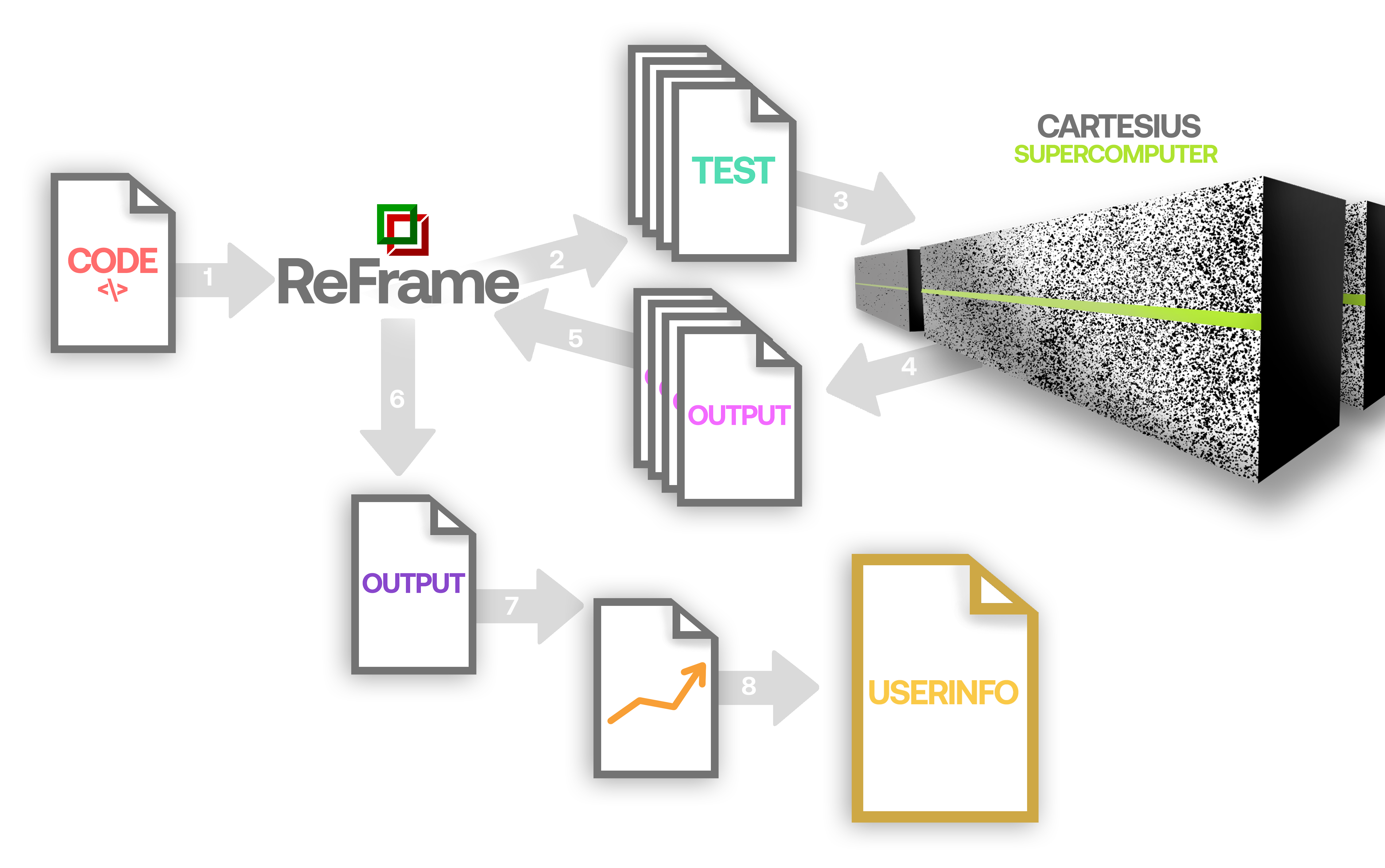
This model is used at the Earth Sciences department as a research tool and as a forecasting model (https://dust.aemet.es). The model uses different datasets as inputs and there is a previous work of interpolating these outputs to a common grid. Furthermore, once the model finishes, the user can retrieve the output in different grid configuration and vertical distribution. To complete all these tasks, the Computational Earth Sciences department has been developing the Interpolation Tool (IT) in Python. This tool uses a wide range of interpolation methods to provide flexibility to the atmospheric scientists.
The goal of the project is to extend the flexibility of the current tool, providing an API to be called from other tools or services, not only stand-alone by the MONARCH model, and decouple the current implementation from external tools as CDO or ESMPy. The candidate will work on the mathematical aspects of the tool and the computational performance to perform post-processes in a big files in an optimal way and improve parallelization, especially regarding the horizontal interpolation, working on techniques of domain decomposition.
Project Mentor: Kim Serradell Maronda
Project Co-mentor: Francesco Benincasa
Site Co-ordinator: Maria-Ribera Sancho and Carolina Olmopenate
Participants: Daniel Cortild, Brian O’Sullivan
Learning Outcomes:
The candidate will work in an operational project, within the Computational Earth Sciences team and will learn how to deal with earth system model outputs in an HPC environments as Mare Nostrum and other clusters, supporting different job schedulers and software stacks. In addition, the student will improve his mathematical knowledge and will learn how to profile and evaluate the computational performance of a given tool.
Student Prerequisites (compulsory):
Python developing skills.
Mathematical knowledge about interpolation methods.
Student Prerequisites (desirable):
Experience with HPC job submission.
Experience with Earth Sciences model formats (netCDF).
Experience as software engineer to develop a custom API.
Training Materials:
Python in High Performance Computing (https://www.futurelearn.com/courses/python-in-hpc) is a great course and will give a very valuable background to the student.
Workplan:
Week 1-2: discover BSC Earth infrastructure, learn to run the tool and explore different use case. Start looking the code to get familiar.
Week 3-4: Gather requirements for the API and start modifying the code to get rid of external dependencies.
Week 5-6: Develop API access and custom interpolation methods.
Week 7-8: Validate results and computational performance.
Final Product Description:
An improved version of the IT tool. This new version will have better performances, improved capabilities, remove external dependencies and will be easier to be used in other tools of the department with interpolation needs.
Adapting the Project: Increasing the Difficulty:
Start coupling the improved IT tool to the other department tools (i.e. Providentia).
Adapting the Project: Decreasing the Difficulty:
Get more support from the research engineers working in the development of the tool and focus only in the first part of the project (modifying the code to get rid of external dependencies and implementing custom methods).
Resources:
The student will have accounts to access the Earth Sciences environment (including access to GitLab, wiki and storage) and an HPC account to MareNostrum and Nord3. Both accounts will be provided by the center.
*Online only in any case
Organisation:
BSC – Barcelona Supercomputing Center
![]()


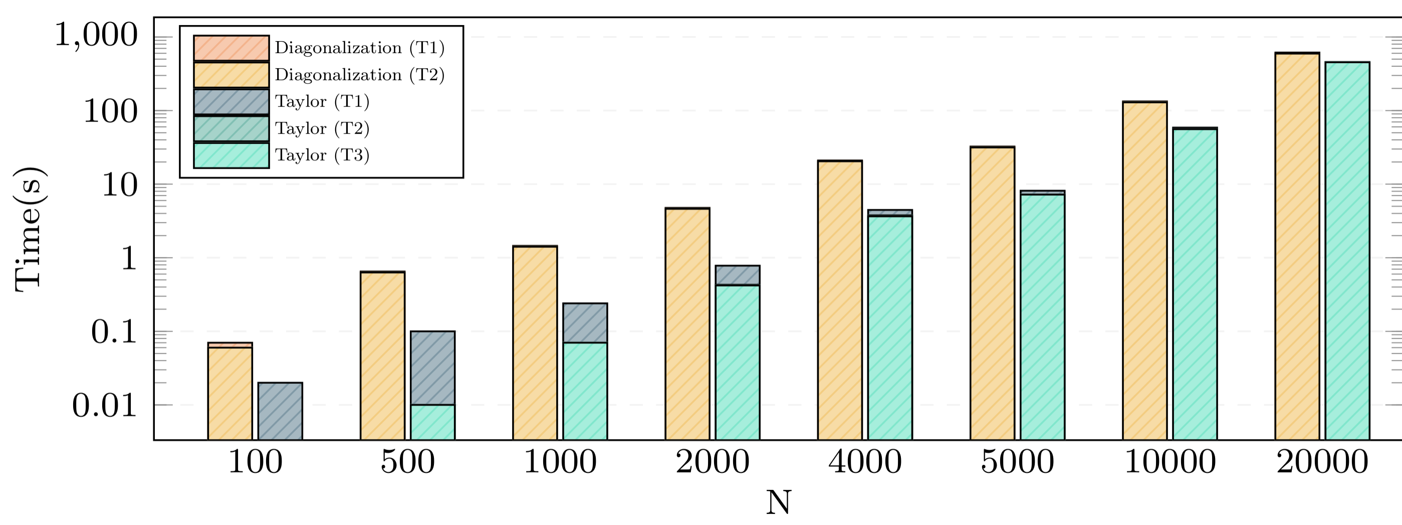
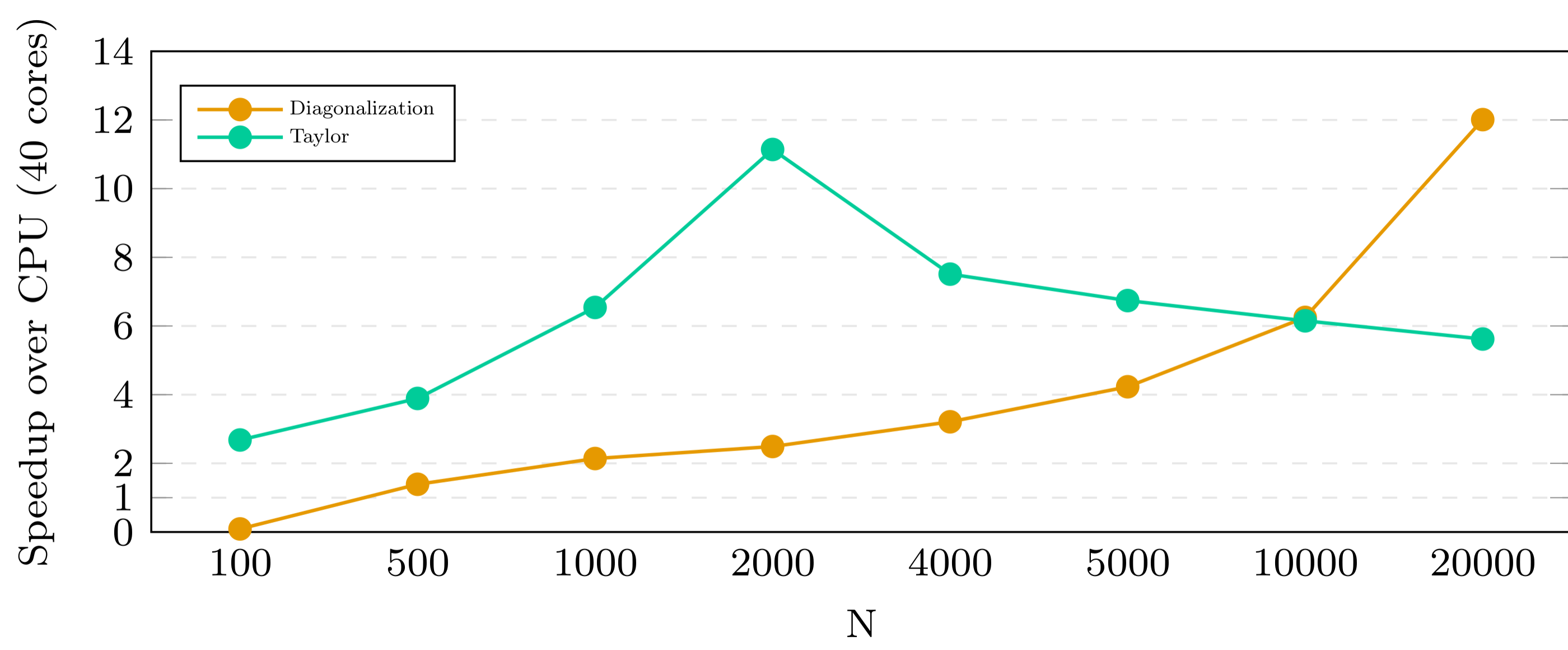


 .
In C++, the function can be written like this:
.
In C++, the function can be written like this:
 but what happens if x is not a number but a matrix? Does the expression
  with a square matrix
  even make sense?
 = \sum_{n=0}^{\infty} \frac{x^n}{n!}") with
with  ,
, = \sum_{n=0}^{\infty} \frac{A^n}{n!}") .
. ,
,  and
and  ,
, ,
, contain the eigenvectors of
 =Q \exp(D) Q^{-1}") .
.") and this matrix is again a diagonal matrix with the exponential of the diagonal entries of
and this matrix is again a diagonal matrix with the exponential of the diagonal entries of ") and
and  , we obtain the matrix exponential of