Applications are open from 18th of January 2019. See the Timeline for more details.
PRACE Summer of HPC programme is announcing projects for 2019 for preview and comments by students. Please send questions to coordinators directly by the 15th of January. Clarifications will be posted near the projects in question or in FAQ.
About the Summer of HPC program:
Summer of HPC is a PRACE programme that offers summer placements at HPC centres across Europe. Up to 20 top applicants from across Europe will be selected to participate. Participants will spend two months working on projects related to PRACE technical or industrial work to produce a visualisation or video. The programme will run from July 1st, to August 31th.
For more information, check out our About page and the FAQ!
Ready to apply? Click here! (Note, not available until January 15, 2019)
As I said in my first blog post, I came from a city called little Amsterdam because of bikes. Therefore it was obvious that I would buy a bike here. I wanted to buy the cheapest bike possible. You can buy some old rusty bike for 50-80 euros from someone. But there was the first shock – I was thinking about Amsterdam as a city where you can let your bike without locking and after two months it will be still there. I was totally wrong. There is a huge problem with stealing bikes. And if you buy a stolen bike, you will have a serious problem. For that reason, I went to the bike shop looking for a second-hand bike. Damn, it is much more expensive. But I was lucky. I found it. 100 euros – “cheapest but one of the ugliest bikes”, as the salesman said. Except for the look, the salesman had to use the hammer to adjust the seat, but it is a bike, my bike now. From that day I‘ve never used public transportation in Amsterdam.
The first day, I discovered the motto of Dutch people: “Why would you be in the traffic jam in your car, when you can be in the traffic jam on your bike”. Most people here go to work with their bike, and you can go everywhere by bike. Amsterdam is owned by cyclists. If you walk on the cycling path they won’t stop and you will be driven over. (Not really, however, I am not going to try that.) They even have separate traffic lights for cyclists everywhere and a lot of underground garages for bikes.
It took me two or three days to adapt to their rules. Because nobody respects the rules here. Is it a red light? No problem. You have right of way and somebody crossing your way? No problem he just accelerates to be faster than you. If you adapt to these unwritten rules you will have a nice time on a bike here.
The opposite story is the city center where most of the cyclist (actually most of the people) are tourists. They don’t know how to ride a bike here and also pedestrians do not respect cyclists there. That’s why I parked my bike in the parking boat every time I went to the city center. Yes, park your bike in a place which is supposed to, otherwise, it is quite possible that your bike will be towed away.
I was cycling to work every day. It was 10 km from where I was staying. If instead I used public transportation it would take me the same amount of time and I would have to pay for it. So it is also a free work-out. If only other cities will be the same.
I would like to start with a joke: Cat walks into a bar… and doesn’t.
That is Schrodinger’s cat which shows us how bizarre the quantum world is. Some people understand Schrodinger’s cat experiment in a way that you can not know if the cat is dead or alive until you open the box. But in reality, this experiment shows that the cat is actually dead and alive at the same time, and after opening the box it defines the state – being alive or dead. So you can actually kill the cat by opening that box. But how can something be dead and alive at the same time? And how can the state change only by looking at it? That is the point of Schrodinger’s idea to point out that the quantum world is completely different from our view of the world. If a quantum particle is in manystates at the same time it is called in superposition between these states.
Now let’s introduce quantum probabilities. To do this, we can use our everyday quantum measurement device – polarized sunglasses. If the photon reaches the polarized filter of sunglasses and it is polarized on the same axis as the filter, it has a 100% chance to go through the filter. Contrariwise, if the polarization of the photon is 90 degrees to the filter, it has 0% chance to go through. And finally, if the angle is 45 degrees it has a 50% chance to go through. So, from 1000 photons, around 500 photons stop and 500 photons go through. But the quantum weirdness is that we can’t actually know before this measurement which photon will come through and which one stops. We only know the probabilities. And of course, the measurement changes the polarization of photons. This quantum non-determinism worried physicists for decades, Einstein commented it with a famous quote “God doesn’t play a dice”. He and many more physicists thought that there must be some “hidden variable” which we have to find, or we can‘t, but still has to be there. But the Bells inequality test experiment showed us that there is no hidden variable.
Quantum entanglement. In the 1930s, Albert Einstein was upset about quantum mechanics. He proposed the thought experiment where according to the theory, an event at one point in a universe could instantaneously affect another event arbitrarily far away. He called it “Spooky action at a distance” because he thought it was absurd. It seems to imply faster than light communication – something his theory of relativity ruled out. But nowadays, we can do this experiment and what we find is indeed spooky. Let’s imagine two entangled photons and we are going to measure them at a 45 degree angle from their polarization. We find out that if we measure them at the same time, in the same direction we get the same result. Both photons stop or both go through. But it is strange that entanglement works on any distance instantaneously. Measuring one photon instantaneously affect the result of measuring the second photon at any distance in our universe.
The quantum internet and quantum computers are based on these strange principles. That is the reason why they are so different from anything we are used to and why we can do things we cant before.
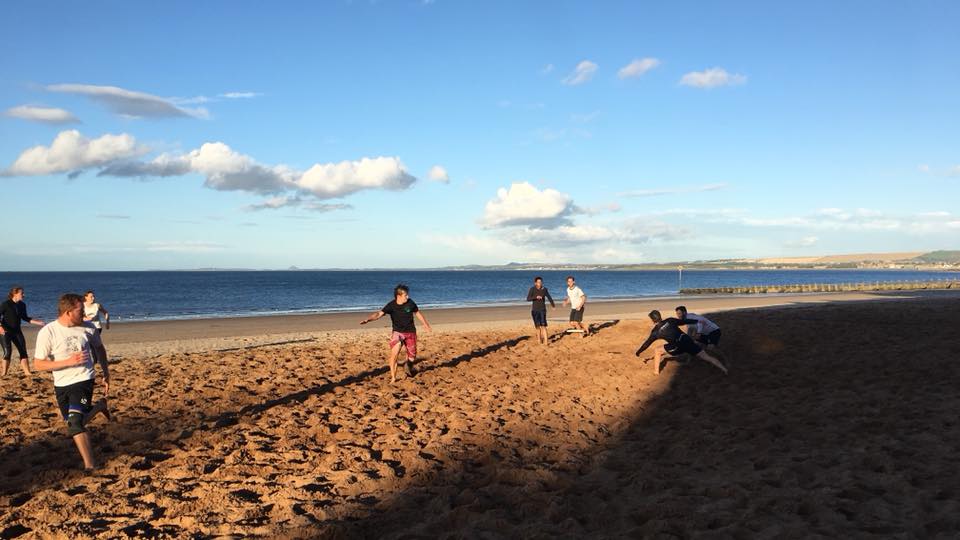
Traveling to foreign countries for longer periods of time is always a great experience, especially because you have a chance to really get to know the culture and to meet new people. Making friends abroad might often be a challenging task, however, it is easy if you play Ultimate Frisbee. If you still believe that playing frisbee means that people just randomly throw a frisbee in a park, you should better check the rules out…. Ultimate as a self-refereed sport is based purely on the Spirit of the Game and because it somehow brings together people with alike thinking it is so easy to make friends. All you need to do is literally shout out Ultimate Frisbee (… and maybe to check local Frisbee Facebook page).
Edinburgh Ultimate Summer League
My first experience with Frisbee in Scotland was a bit hectic. Just on a Tuesday evening I managed to join a pick-up team for the Summer league that was starting on Wednesday. So the next day I went to a park I have never heard of before, to play a match with a bunch of people I have never met before. Guess what? Yeah, we lost the game. Maybe also because we could barely recall each others names. To fix the problem with names and also to supplement the calories burned, we went to a pub for a burger and a beer. Over the next 5 weeks of the League we won 2 games, finished up 4th (out of 6 teams) and consumed dozens of burgers together.
Team White after the last game of Summer League.
Trainings
Selfie with delicous hand-made cookies we got after training.
Twice a week there are regular training sessions happening in Edinburgh. One restricted to women only and the other one open for anyone. These take place at Meadows park, a huge open-access park just in the middle of Edinburgh with a beautiful view of Arthur’s seat as well. Surprisingly, all these trainings had a great quality and we got some highly experienced players to lead the trainings, everything for free.
Beach
Definitely the best part of Ultimate in Edinburgh is the beach. I have mentioned how beautiful Portobello beach in my first blog post and it gets even better if you get to play Frisbee on the beach. If the weather allows, there is a pick-up game happening twice a week, players of all levels are most welcome. As romantic as this sounds it also has a downside. By the end of the game you have sand everywhere, even in your ears usually and even a short swim in the North sea we had after each game does not really help to get rid of it.
Frisbee on Portobello Beach.
My ultimate Ultimate Adventure
After a couple of weeks in Edinburgh, I thought that playing here only is not that adventurous any more and decided to explore the UK Ultimate scene a bit more. A frisbee friend of mine helped me to get in touch with the captain of the Reading womens team and just a week later, I took off from Edinburgh and landed at Gatwick to get a lift with Avril (who I’ve never seen before) to Edenbridge where the tournament took place. So the treat of this summer for me were actually the flight tickets. No regrets at all. It was amazing. Two days of high level Ultimate and unbearable heat, two nights in a sleeping bag on a floor in a Scout Hut, all with people I met for the first time in my life. Unforgettable experience!
After two months of intensive work here in the heart of Scottish pride plains, a time has come to conclude the results and verify the initial expectations.
My project was developed as a part of a data processing framework for Environmental Monitoring Baseline (EMB). The idea is simple: there are plethora of sensors around the UK that measure various environmental indicators such as water ground levels, water pH or seismicity. These datasets are publicly available on the website of British Geological Survey.
In terms of data analysis we are far past manual supervision therefore in addition to the proper dataset labelling and management, there is a need for a robust processing framework that also aids valid data acquisition. The task is fairly simple when we can identify our key needs but this entry stage of targeting the crucial aspects of our future system should not to be underestimated as it tends to have a greater impact the more advanced the work on the system is. Fortunately, environmental sensors, being a part of the IoT world, exhibit some particular characteristics that more or less translate to the nature of the data that will be consumed by our processing framework. Firstly, it can be expected that the data stream will be quite intensive and in the first approximation, continuous – when multiple sensors report every several minutes, the aggregated data flow rate becomes a significant issue. Furthermore, the we need the analysis to happen in the real-time. The third requirement of the system would be that the data might be of use later, therefore it needs to be stored persistently. At last, we need to run our system on HPC because it is Summer of HPC, that’s why. But seriously, systems like these require a reasonably powerful machine to run.
Soa either by extensive search on the web, or by experience, we can relatively quickly find the necessary tools to match our requirements. Whereas we might not be able to pinpoint precisely every aspect, there is no need to worry because we will take advantage of a software engineering paradigm called modularity. In modularity approach we want our software components separated and grouped by functionality, so that we can replace one, that does not exactly fit our needs with a more suitable one later in the project’s timeline. It is very much like creating our tiny Lego® bricks, then grouping and finally putting them together to form a desired shape.
To conclude the above reflections on how important our initial problem identification is, let’s dig into the software-requirement matching phase. All software components are open-sources, with majority of them being released on the Apache license.
Combining the first requirement with the third one, we have a demand for the high-velocity, high throughput persistent storage database. To satisfy this, we can use the Apache Cassandra database which is a column-wide no SQL, distributed database that supports fast write and read, while maintaining well-defined, consistent behaviour. So we can safely retrieve data while we are simultaneously writing to the database. Real-time analysis for HPCs can be managed by using large-scale data processing called Apache Spark that supports convenient database-like data handling. Additionally, Spark code being written in a functional style, naturally supports parallel execution and optimizes for minimal memory write/read – that is especially visible when we use Scala programming language to code in Spark. In order to make our processing architecture HPC ready, reproducible and easy to set up we will containerize our software components. This means putting each “module” in our modular system in a separate container. Containers provide a way of placing our application in a separate namespace. What this roughly means is that our containerized applications will not be able to mess with our system environment variables, modify networking settings or as an another example, use restricted disk volumes. As a bonus, containers use little system resources and are designed to be quickly deployed and run with a minimal system babysitting. Basically, we put our rambunctious kids (applications) in a tiny, little playground (containers) with tall walls (isolated namespace) which also happens to be inflatable so we can deploy it anytime (rapid, automated startup).
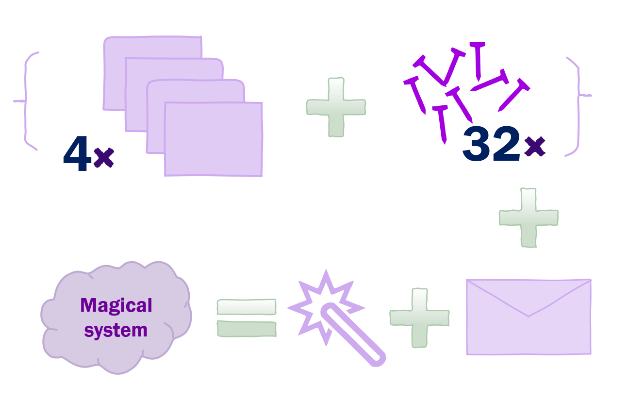
How to build a successful processing system. This useless IKEA styled diagram does not explain it. Idk, just get some containers using basic tools, add some messaging and programming magic and it might work. When it doesn’t, no refunds
Hold on a minute – we have ended up with modular architecture but hey, since everything is written in a different language, uses different standards, how can we communicate all those modules with each other? This is our hidden requirement – the seamless communication across different services and to solve that issue we use Apache Kafka. Kafka is very much like a flexible mailman-contortionist. You tell him to squeeze into a mailbox – done, oddly shaped cat-sized door? – no sweat, inverted triangle with a negative surface? – next, please. Whatever you throw at him, he will gladly take and deliver with a smile on his face (UPS® couriers please learn from that). So in programming terms, we will inject a tiny bit of code into each of our applications – remember, those cheeky rascals sit in the high security playgrounds but we are working on communicating all the playgrounds together so they can transfer toys, knives or whatever else between themselves. This tiny bit of code will be responsible for either receiving messages or sending messages via Kafka or both. Moreover, in order to tame our messy unrestrained communication we provide the schemas which will tell each application what it can send or receive and in what format it has to write or read the data.
By following the breadcrumbs we have arrived to our final draw-out of the architecture. Putting it all into a consistent framework is a matter of time, amounts of coffee and programming skills, but all in all, we have managed to come up with a decent makeup that meets our needs. Shake your hand. You’ve earned it.
I have got a name already — the FåKopp. The name roughly translates to get a cup (of coffe obviously, or scotch since we are in Edinburgh, right?) and relates to the amount of coffeine required to complete the project.
That’s all folks.
Featured image This is a sneak-peak of an actual architecutre
In my previous post I discussed Job Scheduling algorithms, now I will tackle how we are approaching working with them.
In my project, the NEXTGENIO research group (which is part of PRACE) have made a HPC system simulator that allows us to implement different job scheduling algorithms and test their effectiveness, without having to use ARCHER (Edinburgh’s supercomputer), which is expensive to use. It is not a finished project yet and there is still some software engineering to go through, output features to be added and tests to be done. It also had to be made compatible on MAC OS as it had been developed in LINUX, which I did in my first two weeks, this just involved some software engineering.
My supervisor wanted a selectable output feature to be added to the project. Two output types that were developed at the Barcelona Supercomputing centre called OTF2 (Open trace format) and Paraver (browser for performance analysis) were desired to be chosen between to show the output. This has been implemented and been written so that other types can be added to the project too with relative ease.
Simulator design.
Algorithms
Initially, the simulator only had the First-Come-First-Serve algorithm. In this project we strive for better performance, so let’s look at some other algorithms. First off, the score-based priority algorithm which sorts jobs according to scores where we incorporate a fair share scheduling weight to adjust score based on the total number of compute nodes requested by the user, the number of jobs they are running, their recent history and the fraction of their jobs completed. Next, we have multi-queue priority which incorporates numerous queues with different levels of priority and there are certain conditions required to be in each queue. Finally, we have backfilling. Here we opportunistically run low priority jobs when insufficient resources are available for high priority jobs. That’s our list of job scheduling algorithms which sort the order of the job waiting queue. The scheduling algorithm runs on job events such as when a job starts, finishes, aborts or arrives and if there are no events in the past 10 seconds it runs anyway.
The task of mapping algorithms determine which compute nodes to run the job on. The goal is to minimise the communication overhead and reduce cross-job interference. Random mapping is considered the worst case scenario. Round-robin keeps the nodes in an ordered list and when a job ends the node is appended to the list. Over time, the fragmentation of the list becomes significant and the communication overhead drastically increases. For Dual-End we set a threshold value for time which groups every job into short or long. Short jobs search for unoccupied nodes from one end of the list, long jobs search the other end.
Each job has a priority value P(J) with the wait queue being ordered in terms of highest priority. The priority is the sum of five different heuristics. Minimal requirement specifies details like the number of nodes. Aging helps avoids job starvation, and is shown in detail on the right, where age factor is a multiplicative factor of choice. Deadline maximises the number of jobs terminated with a deadline. License heuristics gives a higher score to jobs requiring critical resources on nodes such as NVRAM which hasn’t been implemented yet. Response minimises the wait time for jobs with the shortest execution times by a boost value, which is the backfilling component of this algorithm. This paper goes into good detail about backfilling.
Free time
I’ve been making good use of my time off. First, Jakub and I went up to explore the Royal Observatory on Braid and Blackford Hill beside where we work. The temperatures have been so high here that there were fires on top of the hill and firetrucks were needed to put them out. The observatory was closed when we went up but I think we will revisit and see if we can get to the top.
The Royal Observatory.
Candid photo of me catching some zzzz’s on the hill, taken by Jakub.
Fire trucks on top of the hill, there were bush fires due to the heat.
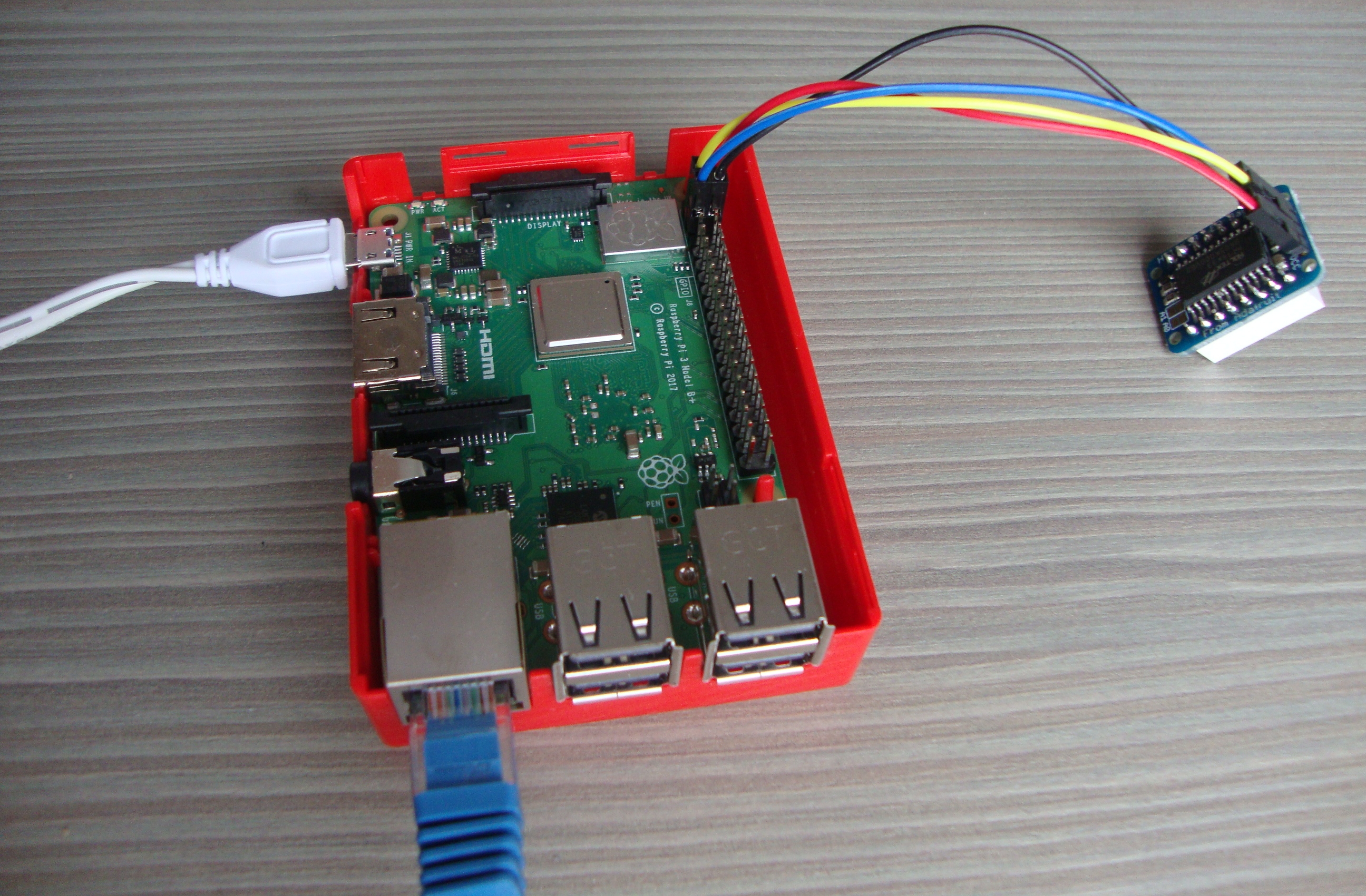
In my previous post I summed up what it is like to build up a Raspberry Pi based “supercomputer”. Since Raspberry Pi is a versatile device there are many more fun things one can do with it besides just running programs on it. One possibility is to connect a small LED lights panel to it to allow, for example, real-time visualisation of computations.
Hardware
All you need besides the Raspberry Pi is a LED Backpack. In my case, for the Raspberry pi cluster I was provided a set of 5 Adafruit Mini 8×8 LED Matrix Backpacks which can be connected directly to a Raspberry Pi:
Adafruit LED Matrix Backpack connected to a Raspberry Pi.
Unfortunately, the lego cases I have for the Raspberry Pis are not quite suited for the use of LED lights, so my small supercomputer does not look that cool any more. It turned more into a random bunch of cables with different colors.
“Supercomputer” with LED lights.
Software
Programming the LED lights might sound difficult at first but it is actually quite simple. The two main pieces of software one needs are:
Freely available Adafruit Python Led backpack library. It is a Python library for controlling LED backpack displays on Raspberry Pis and other similar devices and it provides instructions for both installation and usage.
Python PIL (or PILLOW) library, more specifically Image and ImageDraw modules.
Programming
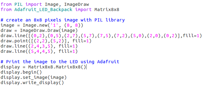
To avoid lengthy explaining of the mentioned libraries, lets have a look at an example straight away. The following piece of code implements one of the basic programs for LED lights which is a simple print of an image that consists of 8×8 – 1 bit pixels:
Python code.
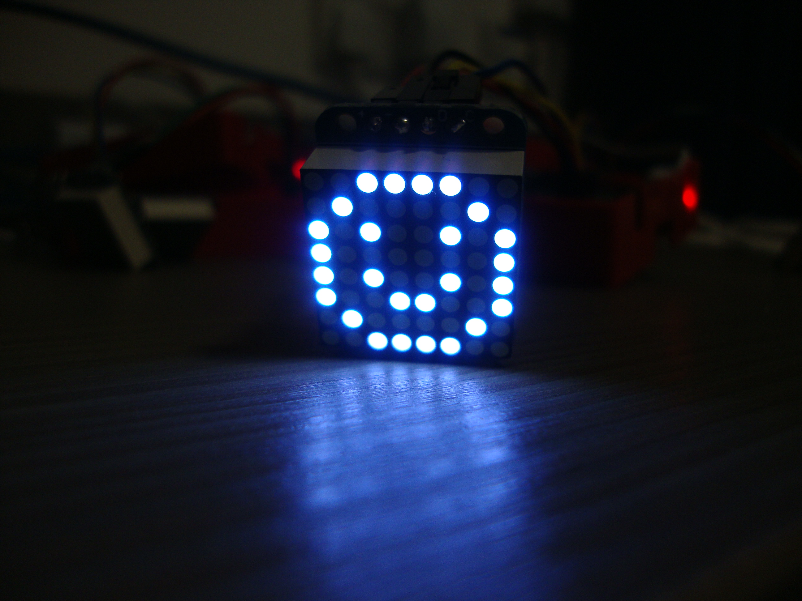
So first, with the aid of the Python PIL library, an 8×8 1 bit image is created and the desired pixels are set to nonzero values using the ImageDraw functions – draw.line and draw.point. Secondly, the LED light display is initialized and the created picture is simply printed on the LED light using the Adafruit Python library functions. As easy as it gets right? Could you guess from the code what the result will look like?
The result 🙂
The Adafruit library provides a few more simple functions such as:
function that sets a chosen pixel of the 8×8 matrix directly to either on or off without the need of creating a PIL image
horizontal scrolling function that: “Returns a list of images which appear to scroll from left to right across the input image when displayed on the LED matrix in order.”
vertical scrolling function that works similarly to the horizontal one but the image appears to scroll from top to bottom
However, there are many other functions that one might find useful, such as rotation of an image or backwards horizontal/vertical scrolling. Even though these functions are not part of the Adafruit library one can quite easily implement them on their own.
Provided these powerful tools, all the rest is up to the users creativity. From my personal experience I would say that programming the LED lights is fun. The best part is the fact that you have a visible result and you can see it almost immediately.
Didn’t understand?, well that served it’s purpose then!
This time I would simply like to boast the awesomeness of my Sensei, here at Cineca, who has been indirectly, gelled with some fascinating and intriguing conversations, teaching me HPC kung fu! Well, it is me grasping more than him actually teaching, but you get my point! His official designation for my project is of Site-Coordinator, but Sensei sounds much more awesome, just like he actually is!
Hello again, this is my 2nd blog for my Journey as a PRAACE Summer of HPC 2018 participant. This time I’ll walk you through the some of the sneak peaks of my work so far, as I have developed, debugged and tested the brand new software called Catalyst, which is a subset of another visualization software called Paraview
What does this do?, well it shows images (results), right off the bat, while you’re simulation is running (in my case a CFD simulation). That means with this bad boy, you could have your initial results just as quickly as possible without having to wait untill the last step of the run.
Just think of this software as another game changer for CFD research and workflows! Before Catalyst, this was not possible. Which is why I get to be the lucky one to test it with a full scale – use as many cores feasible – SuperComputer level- HPC test case. So that researchers, academics , or just another curious nerdy kid, could later easily post process their setups, making their life easier. Amazing, right!
As to what exactly I am running. That is an injector which is slightly different than the ones used in car, but it is a model after all! And also the damBreak Case of OpenFOAM which comes in default with the software. Both of them have two phases of fluid involved. So we basically at the end of our test, observe to see one fluid morph into other as time proceeds.
Easier said than done, there are the following elements involved, if I need to test this right.
1) The CAD aspect, (the geometry and mesh should be correct, as is required for any CFD setup)
2) The OpenFOAM aspect, this sets up the geometry or rather the mesh, to be specific. The solver, think of it as a fancy calculator that solves big equations, and output details i.e to say how often do you want your results to be stored and so on. All of which, of course should be set correctly if one wants to avoid the “Garbage in, Garbage out” results!
3) The HPC aspects would involve:
a) The supercomputer, which is the giant tool that actually does the operations and calculations mentioned above, in parrallel.
b)Its access, so that you don’t have to wait in line for your calculation.
c)Your partition, or the place where you run your job on a supercomputer, must have enough resources, like the processing power and so on.
d)The installed and supported packages (so that apples are calculated with respect to apples and oranges with respect to oranges).
The last aspect is especially important because that’s what I am here for. When you have an OpenFOAM job to be submitted to a cluster, the software that works with OpenFOAM , namely Paraview, has been widely tested and appreciated. What has not been tested is the Catalyst side of it. A fairly recent development of sorts, and hence the necessity for its research.
So it is obvious to run into an error every now and then , which may come from any of the above mentioned aspects. And because such a testing is being done for the first time, the number, instances, flavour and variety of errors encountered, increase even more. Mind well, these aspects, in actuality, have much complex dependencies with one another as well as among themselves than what is mentioned.
So the other day, I was couple of hours in, fixing this error I’ve got. “Attribute error: Name not defined”. To give you a context, if one wants to find the vorticities of a flow in this software, a filter would be required, which filters out only the required calculation needed to compute vorticies. And it didn’t seem to work, no matter what I tried.
So, my Sensei comes in and asks for the updates, I brief him about the developments uptill now, and he smiles and tells me that this error was not up for me to fix!!. Turns out, the feature didn’t exist in Catalyst’s current edition (as of 10.08.2018) , and had to be edited in the current edition with a patch file, then recompile it again for the cluster, and then install afresh for this feature to work.
This is when I see the HPC kung fu of my Sensei. He very calmly does the above one by one, explaining to me what’s going on along the way. Few steps extremely intricate because the supercomputer already has many versions of some packages/softwares already installed, which he must navigate through and adjust accordingly, mentally keeping a tab on where he needs to change a setting if required and simultaneously foreseeing any dependencies that might affect at a later stage of compilation.
And then after 2-2.5 hours of tweaking, (remember compiling the whole software again is a lengthy process), the thing is installed (well the workaround at least). Oh and did I mention, it worked in the first attempt.
Just check out the preliminary results!!
I may be stating the obvious here, but to just see him do his jam, was very thought provoking. I may have just scratched the surface of how much consideration goes into software development, especially when you do it on a HPC scale, just by watching him. I’ve never had a mentor before, let alone a one on one mentor. And I must admit, to be striving toward a goal with a mentor is a whole different ball game. The one which you have already won, because you have learned so many things.
Which is why I appreciate so much, that I got this wonderful opportunity to work at Cineca on this project. Those simple conversations that are the by product of his experience, and his wisdom are simply amazing. I at least for one, always look forward to strike up a conversation with my Sensei, just to see what new thing I might acquire in the process!
I perhaps wouldn’t have been able to acquire and learn so many things, if it were not for him. The least I could say is
Arigatto Sensei!!
To deal with QCD, we take a four dimensional space-time lattice and let it evolve step by step until it can be considered to be in thermal equilibrium and then take a snapshot every n-th or so step to get a set of lattices (called a Markov chain) to do measurements on.
So why does this require supercomputing?
Well, to start with, we are not satisfied with just using a small lattice. Nature happens to take place in a continuum and the introduction of a lattice also introduces errors, which get worse as you take smaller grids. So lets take something reasonable like a size of 8 for each space dimension and 24 for the time (which still is quite small). That way you already have 12288 points and on each of those lives a Dirac spinor of another 12 complex-numbered entries. Now, to let the lattice evolve, we need to, as always, calculate the inverse of a matrix, which contains the interactions between all points. So this is some kind of 147456×147456 monstrosity (called the Dirac matrix), which is thankfully sparse (we only consider nearest neighbor interactions). Oh, and all of this needs to be done multiple times per evolution step. So supercomputing it is.
But to deal with the above, we still need to introduce some trickery. For example, one could notice that you can distinguish between even and odd lattice sites like on some strange, four-dimensional chess board. Then you only interact by nearest neighbor with sites of the same color, which allows you to basically halve the Dirac matrix and deal with even and odd sites separately.
Also, you do not save the entire Dirac matrix, only the interactions between neighbors. These are described by SU(3) matrices, which are quite similar in handling to the 3D rotation matrices your gaming GPU uses to rotate objects in front of your screen. With the introduction of general purpose GPUs, this probably has become an exclusively historic reason, but it sure helped to get some speed up in the early days.
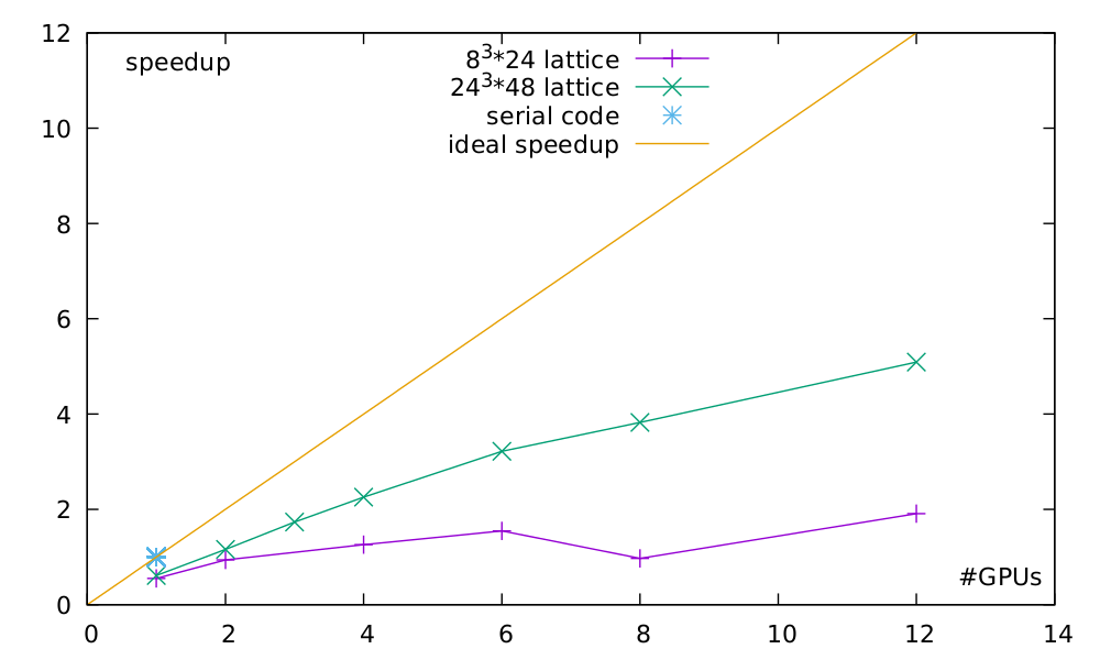
But we talked enough now, lets look at some speedups!
Speedup comparison between a smaller and a medium sized lattice.
As you can see, using parallel code is quite pointless for small lattices. It even gets worse at eight GPUs since you need to have a second dimension parallelized to support that many nodes (Yes, distributing 24 sites on 8 nodes would still work, but you need an even number of sites on each node.). But lo and behold, look at the speedup once we use a reasonable sized lattice. This is how we like it. Not a perfect speedup, of course, but sufficiently working and just waiting to be tuned.
So lets see how well this baby performs at the end of the summer and stay tuned for the next update!
Bratislava is a great city. The first thing that caught my attention when my airplane landed at Bratislava airport was the big green landscapes. The first impression of the city was really great and I couldn’t wait to explore the city. The first days I was introduced to the people in the Slovak Academy of Science in which I was working for my project. They were willing to help me and answer all my questions, not only related to the project, and I learned a lot from them during my stay. I also visited the center of the city which is beautiful with huge and impressive buildings, but the best part is that on one of the bridges that crosses the Danube river, there is a tall construction that people call it UFO, because its shape looks like an UFO, from which you can get a beautiful view and see the whole city. Fillip, who is the head of the HPC in Bratislava, organized a canoe trip along the Little Danube, which is a branch of the Danube, for us and all the people in the HPC center that wanted to participate. We started our journey round 10 am. Canoeing through the forest, in a beautiful river was a unique experience for me because I have never done something similar. I would describe the feeling as hiking with your hands. It is actually pretty similar only at the end of the trip, your hands are the ones that are burned out rather than your legs. The trip was six hours long and we covered more than 20 enjoyable kilometers. Overall, my experience in Bratislava was very good and I am happy that I got to meet such kind people and I am looking forward to visiting the city again to see the places that I missed during this summer.
Grey cast iron, white cast iron, ductile iron, malleable iron,……. Oh my gosh, so many types of cast iron! What is the difference? This was the question which always used to annoy me when I was graduating as a mechanical engineer. Well, the differences are in the chemical composition and the physical properties. All of the cast iron types tend to be brittle but there is one of them which is malleable. Yeah you have guessed it right, it is the malleable iron which has the ability to flex without breaking. Malleability is a common term used in material science and manufacturing industry and is defined as a material’s ability to deform under pressure. But can a HPC application be malleable too? This is the question I am tackling within my project in the PRACE Summer of HPC programme.
Polycrystalline structure of malleable iron at 100x magnification (Source: Wikipedia)
I had no idea that the term “malleability” is also being used in the HPC jargon until I started working on this project. Soon I came to know that like malleable materials, codes running on supercomputers can also be dynamically hammered into whatever size and shape we want. Many times, we have a lot of jobs submitted to the supercomputer, but because they can’t fit into the available compute nodes, they keep on waiting in the queue for long time. This reduces the throughput of the cluster and also the users have to wait longer to get the results. But if the already running jobs can be resized dynamically, then they can allow other incoming jobs to fit in the cluster and expand or shrink according to the available resources. More throughput and lower turn-around time can reduce the cost of the HPC system. Isn’t it amazing? To look into this problem, let’s have a glimpse on the basic categories of jobs according to their resize capability.
Five categories of jobs
Rigid: A rigid job can’t be resized at all after its submission. The number of processes can only be specified by the user before its submission. It will not execute with fewer processors and will not make use of any additional processors. Most of the job types are rigid ones.
Moldable: These are more flexible. The number of processes is set at the beginning of execution by the job scheduler (for example, Slurm), and the job initially configures itself to adapt to this number. After it begins execution, the job cannot be reconfigured. It has already conformed to the mold.
Evolving: An evolving job is one that can dynamically request its resource requirements during its runtime. The job scheduler then checks whether the requested resources are available or not and allocates or deallocates the nodes according to the request.
Malleable: Now comes the fourth type, the jobs which are malleable. These can adapt to changes in the number of processes during their execution. Note that, in this case, it is the job scheduler that takes the decision to resize the jobs in order to maximize the throughput of the cluster.
Adaptive: This kind of job is the most flexible one. The application can itself take decisions whether to expand or shrink, or it can be hammered by the job scheduler according to the status of the available resources and queued jobs.
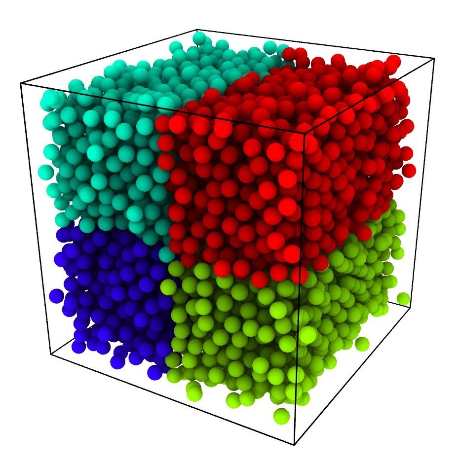
Malleability seems conceptually very good, but whether this scheme works in the actual scenario? To answer this question, I needed a production code to test it. So my mentor decided to use LAMMPS, to test malleability. LAMMPS stands for Large-scale Atomic/Molecular Massively Parallel Simulator and is being maintained by Sandia National Laboratories. It is a classic molecular dynamics code which is used throughout the scientific community.
A dynamic reconfiguration system relies on two main components: (1) a parallel runtime and (2) a resource management system (RMS) capable of reallocating the resources assigned to a job. In my project I am using Slurm Workload Manager as RMS, which is open-source, portable and highly scalable. Although, malleability can be implemented by only using RMS talking to the MPI application and using MPI spawning functionality, but it requires considerable effort to manage the whole set of data transfers among processes in different communicators. So, it was better to use a library called DMR API [1] which combines MPI, OmpSs and Slurm which substantially enhanced my productivity in converting the LAMMPS code into malleable, thanks to my mentor for developing such a wonderful library.
The most time-consuming part of my project was to understand how LAMMPS work. It has tens of thousands of lines of code with a good online documentation. But once understood, it was not very difficult to implement malleability. In fact, it only needed few hundred lines of extra code using DMR API.
I can show you a basic rendering of malleable LAMMPS output. The color represents the processor on which the particles reside. The job was set to expand dynamically after every 50 iterations of verlet integration run. The force model was set to Lennard Jones and rendering was done using Ovito.
I am now in the end phase of my project, testing the code and getting some useful results. In the next blog post, I will show some performance charts of malleability with LAMMPS. I leave you here with a question and I want you think about your HPC application – Is your code malleable?
References:
[1] Sergio Iserte, Rafael Mayo, Enrique S. Quintana-Ortí, Vicenç Beltran , Antonio J. Peña, DMR API: Improving cluster productivity by turning applications into malleable, Elsevier 2018.
[2] D.G. Feitelson, L. Rudolph, Toward convergence in job schedulers for parallel supercomputers, in: Job Scheduling Strategies for Parallel Processing, 1162/1996, 1996, pp. 1–26.
What is a HPC system ? High performance computing (HPC) is the use of parallel processing for running advanced application programs efficiently, reliably and quickly. Typical users are scientific researchers, engineers, data analysts.
In the race for Exascale supercomputer systems, there are significant difficulties that limit the efficiency of the system. Beyond all of this, Dennard’s scaling up energy and energy consumption through the end is beginning to show its impact on limiting the highest performance and cost-effectiveness of supercomputers.
A new methodology based on a range of hardware and software extensions for fine grained monitoring of power and aggregation for rapid analysis and visualization is presented by researchers. To measure and control power and performance, a turnkey system that uses the MQTT communication layer, NoSQL database, precision grain monitoring, and future AI technology is recommended. This methodology has been shown to be an integrated feature of D.A.V.I.D.E. supercomputer.
D.A.V.I.D.E. consists of 45 nodes that are connected efficiently. Infiniband EDR 100 Gbytes network connection, the highest performance of 990 TFolt total and estimated power consumption less than 2 Kwatt per node. Each node is a 2 Open Unit (OU) Open Computation Project (OCP) form factor and hosts two IBM POWER8 Processors with NVIDIA NVLink and four Tesla P100 data center GPUs and has an optimized internal node communication scheme for optimal performance. It stands at # 440 of the TOP500 list and # 18 at GREEN500 November 2017 list.
Energy Efficiency is one of the most common problems in the management of HPC centers. Obviously, this problem involves many technological issues such as web visualization, interaction with HPC systems and timers, large data analysis, virtual machine manipulations, and authentication protocols. Obviously, data analysis and web visualization can help HPC system administrators. To optimize the energy consumption and performance of the machines and to avoid unexpected malfunctions and abnormalities of the machines.
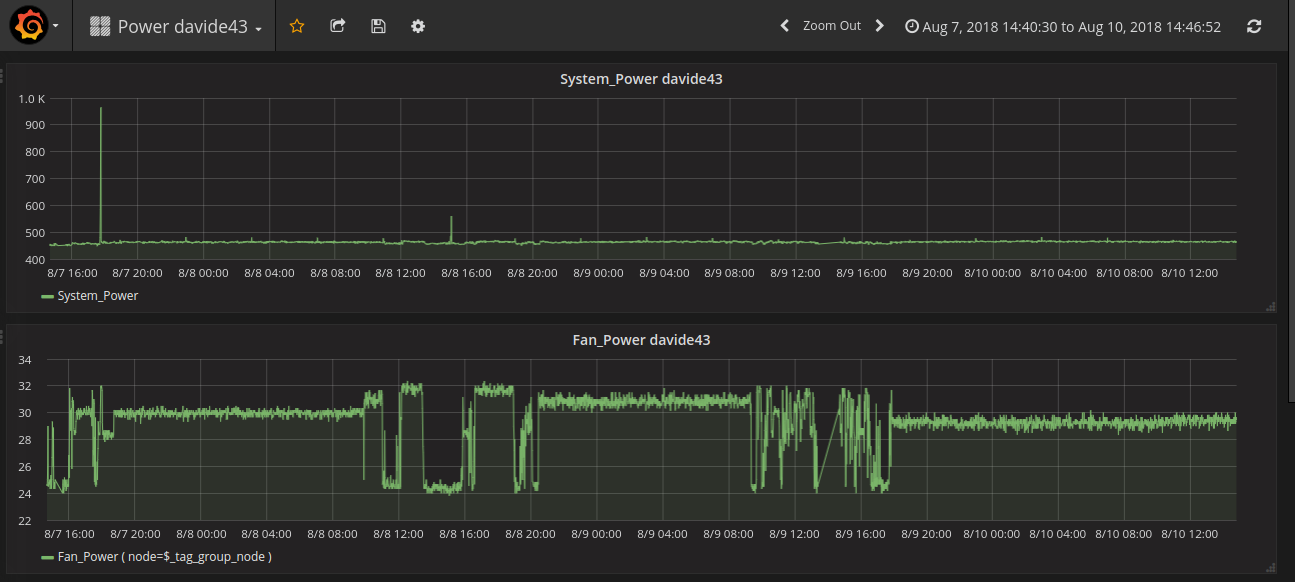
Some example grafhs on the Grafana
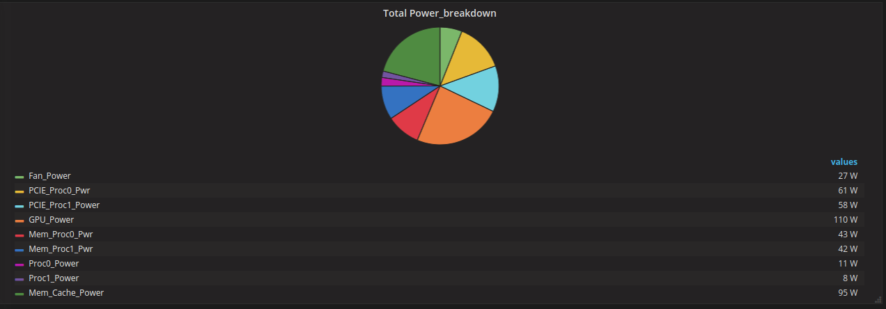
Grafana is one of the tools used for data analysis and web visualization and Grafana is open platform for beautiful analytics and monitoring and general purpose dashboard and graph composer. Grafana supports many different storage backends for a time series data (Data Source). Each Data Source has a specific Query Editor that is customized for the features and capabilities that a particular Data Source exposes. Although the use of Grafana seems a bit complicated, you will see that they will simply describe everything you’ll need when you follow the proper documentation. The link for youis : http://docs.grafana.org/
How I can use Grafana ? D.A.V.I.D.E has two databases ; Cassandradb and Kairosdb. Kairosdb is set up for Grafana as a datasource. Basically I can connect to the Grafana server and create and manage my dashboards from my script. Firstly I managed my dashboards as running dynamically. Also I need to managed them as statically. Because as statically without data source. I can visualize results of more data that doing that it is possible to use snapshot for grafana.
visualization Fan Power and System Power for Node davide43 as using line graph
visualization total power of all metrics separately for nodes which has a job with using pie graph
This Friday the JSC’s summer students arrived, which meant that I was able to tag along for their introductory tour of the Jülich Föreschungszentrum. We cycled around the campus with our guide, Irina Tihaa, a PhD student studying “neuroelectronics”. I wanted to hear a bit more about her field, so she kindly agreed to sit down with me after the tour for a small interview! So what is her group actually studying?
PhD student Irina Tihaa and me after our tour.
“In our institute we are mainly doing electronics for the brain. This is mostly fundamental research; we look at which kinds of materials and electronics we can use, how can we listen to the brain and understand the signals it is sending, and how can we communicate with the brain, via these electronics. First of all, we need to work on the different electronics, but we also need to understand the language of the brain. I’m working mostly on the latter.”
And what kind “medium” is this communication done across? What kind of data is involved?
“A typical example would be that we take a chip, with lots of electrical channels. We cultivate our cells on top. Neuronal cells communicate via electrical signals, so then we can measure the voltage difference across our chip. I also have a lot of optical data. You can introduce fluorescent sensors into the sample, which are activated by light and also emit light. From this you get a lot of video data, because you’re measuring the difference of the intensity.”
Quite an inter-disciplinary field! I asked Irina about the kinds of scientists she works with during a typical week
“In my institute we are mostly physics actually, because we’re a bio-physics institute located in a physics department. We have some biologists, we have some nanotechnologists, we have quite a lot of chemists… Bio-medical engineers… Some medics also, and electrical engineers of course. And then software developers! Almost all of our electronics is institute-made, which means we need software developers and a lot of electrical engineers to construct it. When it comes to analysing the data, because neuronal communication is quite complex, we need complex algorithms. I don’t have the background for this, so I also talk to people from the computational neuroscience institute, who have the expertise to create these algorithms for analysing neuronal signals.”
The research center’s fire brigade at our guest house after someone’s cooking was slightly distracted…
And these kinds of interactions are not at all uncommon at the FZJ. During our tour, every stop reminded me why research facilities with different institutes and people from different fields are so important. Nuclear research means that there is a fire station and highly trained guard dogs on campus. Those dogs also help us forgetful scientists by tracking lost keys when needed! Medical engineers are helping the biology department to do MRI scans of live plants. And as it turns out, Irina’s institute, like mine, also has a graphene connection! Some of the chips she and her team have been building have used graphene. As a carbon-based material, she told me it is chemically quite suitable for our carbon-based bodies. But how does one start studying a field like “neuroelectric interfaces”? It’s hardly something that you come across during your high school or bachelor studies. I was very curious to hear about Irina’s path to Jülich.
“Originally I’m from Kazakhstan, but I’ve been living here in Germany for long time, over 20 years. I was always impressed by the natural sciences; physics, chemistry, biology, mathematics… But the brain kind of impressed me the most, because at some point I realised that even small changes can affect behaviour so much! Like if one part of the brain is growing faster than another during puberty for instance, this can lead to aggressive behaviour. Then it’s changing back, because the other parts are taking back control. This really fascinated me, so I decided to study biology, with a focus on neurobiology. I still had a lot of interest in the other sciences, like modulation, simulations, and physics, so when I met my professor and saw this institute, I realised it was perfect, because there is everything: chemistry, biology, nanotechnology (with physics inside), and engineers working on the electronics. I can really introduce my point of view there.”
And of course, data analysis and and simulations require computers. But not quite on the HPC level yet!
“Up to now we are working more on the smaller level. The simulations that we’re running are a maximum of few days on a very-good “normal” computer. But this is just the beginning. Right now, we’ve been mimicking brain parts on a chip, so in 2D. But we want to of course go 3D, since the brain is three-dimensional! Maybe you have heard of “organoids”, small structures that are similar to the organs we have? And they’re in three dimensions. As you get data from three dimensions, simulations of course get a lot bigger. So at some point also the super-computer will probably be involved.”
I ended by asking Irina if she had any “words of wisdom” for young people considering the sciences.
“I would encourage it, because first of all it is the future! Earlier, we had experiments and we had theory. These were the two pillars of research. But now adays we have this third new pillar, simulation science, which is getting more and more important, and I think it will play a big role in the future!”
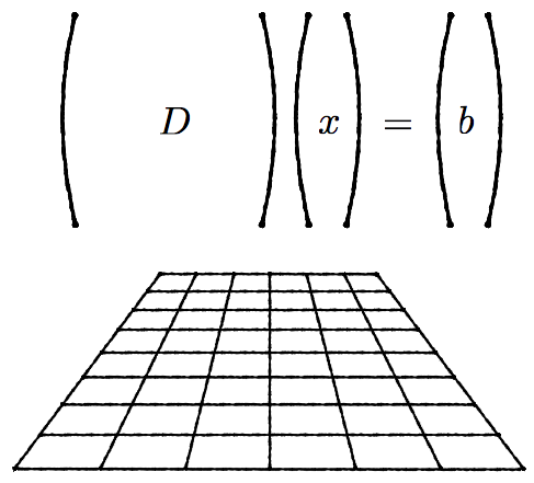
Welcome back everyone! Finally, we are ready to talk about the project. Recalling what I said in my previous post, when doing lattice QCD simulations, I said that we need to “let evolve” the quarks. More precisely, we need to compute the propagators of the quarks from one point of the grid to another. This is done by solving the following linear system:
Let’s explain what each element means: D is the Dirac matrix, which contains the information about the interaction between the quarks and the gluons; b is the source, which tells us where we put the quark at the beginning; and x is the propagator, what we want to compute.
Naively, one would have the temptation to solve this problem by just doing x=D-1 b. But if I tell you that the Dirac matrix is usually a 108 x 108 matrix with a lot of elements equal to zero (sparse matrix), computing the inverse is not an easy step (almost impossible).
There are multiple methods that can handle this type of matrices (BiCGStab, GMRES, …), but the one that we are interested in is the multigrid method.
With this method, as its name says, we create multiple grids: the original one (level 0), and then coarser copies (level 1, 2…). If we want to move between different levels, we use two operators: the prolongator (from coarse to fine) and the restrictor (from fine to coarse). For example, if we apply the restriction operator on the system, we get a smaller grid, which means that the matrix D is going to be smaller, so it will be easier to solve:
Schematic representation of the multigrid method.
After solving the reduced system, we have to project it back to its original size using the prolongator. The construction of these projectors is not trivial, so I won’t go into details, but it requires a lot of time to construct them (comparable to the time it takes to solve). So, to sum up, the steps are the following:
Construct the projectors.
Start with an initial guess of the solution, and do a few steps of the iterative solver on the fine grid (called pre-smoothing).
Project this solution to a coarser grid, use it as an initial guess, and solve the coarser system (should be easy).
Project it back to the original grid, and do some steps of the iterative solver (called post-smoothing).
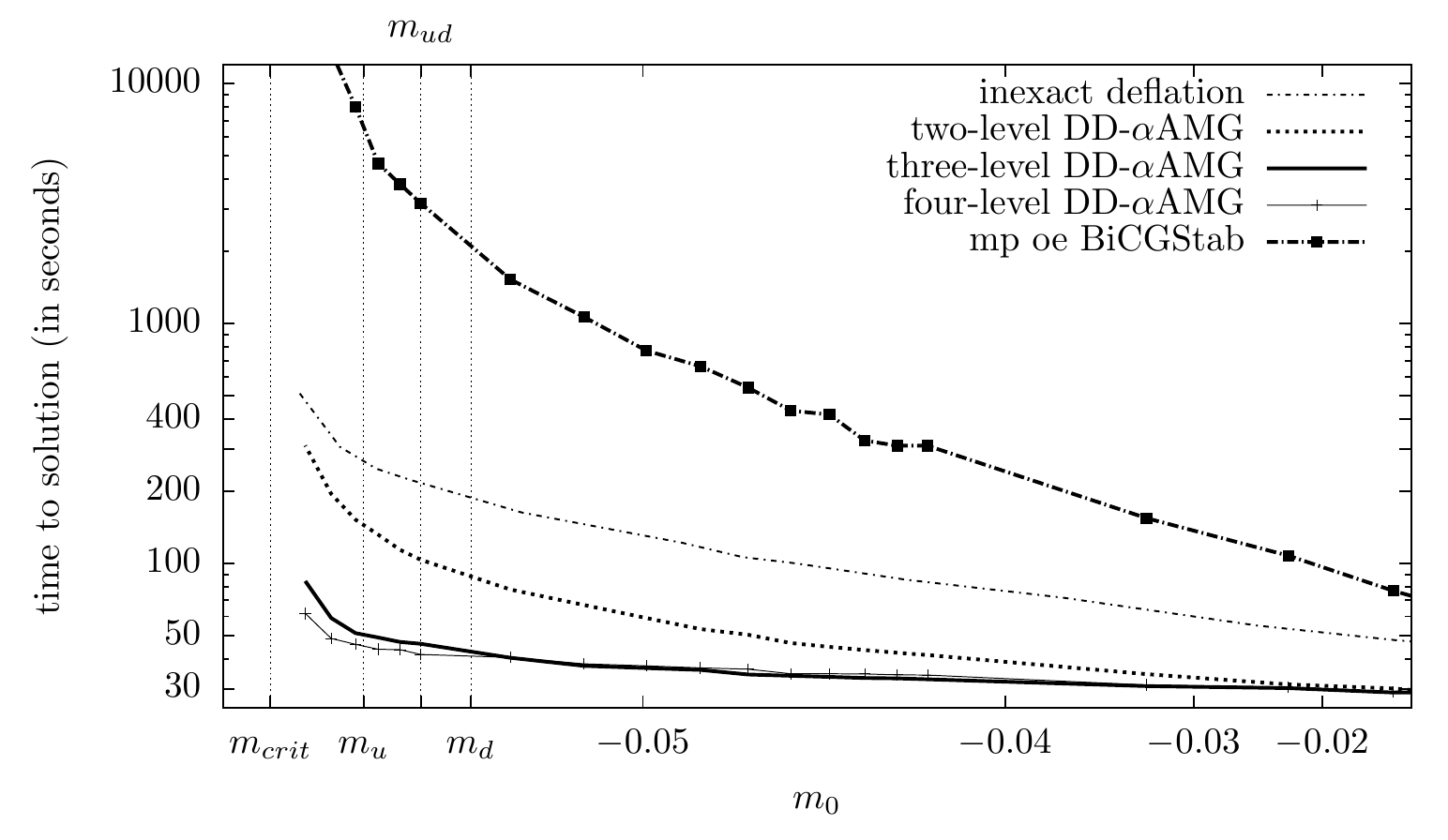
To convince you that this algorithm really increases the speed of the solver, let me show you a plot comparing different methods:
Mass scaling of diferent methods, comparing the time it takes to compute a propagator [1].
Looking at the plot, as we decrease the mass of the quarks (x-axis), the time it takes to solve increases (the y-axis is logarithmic!), but compared to the other methods, the multigrid (the one labelled as DD-αAMG) is always the fastest one, in particular at lower values of the quark masses (the physical values for the up quark is labelled as mu, and for the down quark is md).
So, if the multigrid method is already fast, what can I do to make it even faster? The solution is pretty simple, and it’s the main purpose of my project: instead of solving the linear system for one b at a time, solve it for multiple b‘s at the same time. And how is it done? You’ll have to wait for the next blog post to learn about vectorization, which consists, in a nutshell, in making the CPU apply the same operation simultaneously to more than one element of an array. Cool, right?
Much has been going on here in Athens, as I have now delved into my project. I’m studying the effects of the E545K mutation of the PI3Kα (phosphatidylinositol 3-kinase α) protein using molecular dynamics with enhanced sampling techniques, in particular metadynamics.
The protein PI3Kα is an enzyme that, upon binding to membrane proteins, catalyzes the phosphorylation of phosphatidylinositol bisphosphate (PIP2). The product of this reaction (PIP3) then participates in a cascade of intracellular communications that has implications in cell growth, metabolism, survival, etc. Because of the key role of PI3Ka in promoting all these processes, mutations in this protein are actually the most common protein mutations that lead to the development of cancers. The E545K mutation in particular causes the disruption of interactions between two domains of PI3Kα, facilitating the detachment of theses domains from one another and leading to overactivation.
Detachment of helical and sNH2 subunits of the PI3Kα protein with the E545K mutation. The wild-type protein would have aminoacid 545 as Glu instead of Lys.
Knowing exactly the effects that the E545K mutation provokes at the molecular level is fundamental to develop drugs that can target specific structures in the protein and prevent the overactivation that leads to cancer. Molecular dynamics simulations can help towards accomplishing this goal, as they provide a detailed atomic description of the dynamic evolution of the mutated protein.
However, standard MD simulations, even on modern hardware and large clusters, can only achieve timescales of up to microseconds. This is not enough to study large protein domain movements such as the one we’re interested in. This is where metadynamics comes in. It is a way to more efficiently explore the energy surface of our system, in order to arrive at relevant stable (minimum energy) configurations that describe our process, along predetermined geometric/functional variables (so called collective variables).
Sounds complicated, but let me describe the basic principle with an analogy. Imagine you are Noah, and you are stuck in a valley with the Ark, having already saved all the animals in there. You can’t push the Ark out of the valley by yourself of course, the mountains are impassable. But then God lends a hand. He starts filling the valley with water. Suddenly, the Ark starts floating and keeps going up. Finally, when that valley is completely flooded, you are able to surpass the mountains, into the next valley. You explore this new valley, saving all the creatures in there. Then God repeats the process, filling in that valley and allowing you to escape to the next one. After a while everything will be flooded, but there will be nowhere left to explore either. I refer you to this excellent Youtube video where you can observe what I just described in a simple way.
In this analogy, the valleys are the energy minima of our system, and the Ark is our MD engine, which allows us to explore the “energy landscape”. Metadynamics is the flooding process: in technical terms Gaussian functions are constantly added to our original energy surface, preventing us from being stuck in the minima surrounded by very large energy barriers (“mountains”). It’s a very powerful method, and has various parallel implementations as well. I’ve been analyzing results from metadynamics simulations already made, and I’m setting up a simulation myself to run on ARIS.
I leave you with another picture from my various trips across Athens, this time an incredible view of the city from the top of Mount Lycabettus. See you next time!
The official title of my project is “Parallel Computing Demonstrations on Wee ARCHIE”.
Wee Archie
One would therefore probably expect me to be spending most of my time playing around withWee Archie. For those who don’t know yet, Wee Archie is a small portable suitcase-sized supercomputer that is built out of 18 Raspberry Pi. EPCC uses it to illustrate how supercomputers work to a general audience. It has become so popular that it is quite hard to get to working with it now. Therefore, to be able to develop new applications for Wee Archie, my initial task was actually to build a smaller version of Wee Archie on my own.
What is needed
On the very first day at the EPCC, my co-mentor Oliver gave me a box full of stuff and told me that everything I need to build a Raspberry Pi cluster is in there. Also, he said that a ten year old kid can do it so it should not be a problem for me. This is what was in the box:
All you need to build a small cluster.
set of 5 Raspberry Pi B+ (quad core) with power cables
5 lego-compatible Raspberry Pi cases
ethernet switch
6 ethernet cables
5 micro sd cards with adapters
HDMI cables (useless if you dont have a monitor to connect to)
Building the cluster
To be honest, Oliver was right. Physically building up the „cluster“ is really easy, provided you read the instructions carefully step by step. Not doing so might have some unpleasant consequences. My beloved friend James summed up my experience nicely into a meme:
A take-home message? Raspberry Pi has no build in memory and trying to “ssh” to it without plugging in an SD card with an operating system will highly likely not be successful, no matter how hard you try.
Networking
The network setup however, was a bit more challenging of a task, especially when using Ubuntu and the very first instruction part for Linux only said: TODO. Luckily, Raspberry Pi seem to be so popular, that Stack Overflow and other geek forums have answers to literally any problem one can have with them. Otherwise, the instructions were quite clear and now I believe that a smart ten years old kid could do it on their own within a couple of hours. For pure mathematicians like me, it might take a bit longer, but two days later I finally had a working “supercomputer” connected to my laptop.
Running programs
Once all the setup is done, running programs on a Raspberry Pi based cluster is no different from doing it on a standard cluster. Except, maybe, the fact that running a parallel program on all 20 cores of this small “supercomputer” is still slower than running the same program sequentially on a standard laptop. The performance is however not what we are looking for with such a cluster. It’s the fun one can have playing around with this cute device, such as running the parallel “windtunnel simulation” that EPCC developed and now uses for outreach purposes:
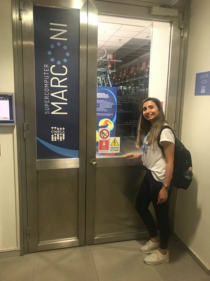
Hi from Bologna ! 🙂 It has been 5 weeks since I came to Bologna.
It is a small and enjoyable city. I stay in the center of the city. CINECA, Italy’s HPC center is a bit far off the center. I use the bus to go to CINECA every day during the week. Bologna is a different city with its houses and ways. The houses have an old structure and are in general colorful. It is famous for delicious foods such as pasta, pizza and ice-cream – all of which I have tried 🙂 I think Special Bologna pasta is the name of their spaghetti bolognese – which for me is the best. Bologna is a musical city like other European cities and I always see someone who plays an instrument in the centre when I return. It makes me smile. People who live in Bologna are very helpful and cheerful. The city has no more tourists so it makes it calm.
Spaghetti Bolognese !
CINECA is a non-profit consortium and made up 70 Italian universities. It is established in Casalecchio di Reno, Bologna and hosts the most powerful supercomputer in Italy as stated in TOP500 list of the most powerful super computers in the world. One of these is Marconi composed of Intel Xeon Phi’s and is ranked at the 14th position of the list as of June 2017, with about 6 PFLOPS of power.
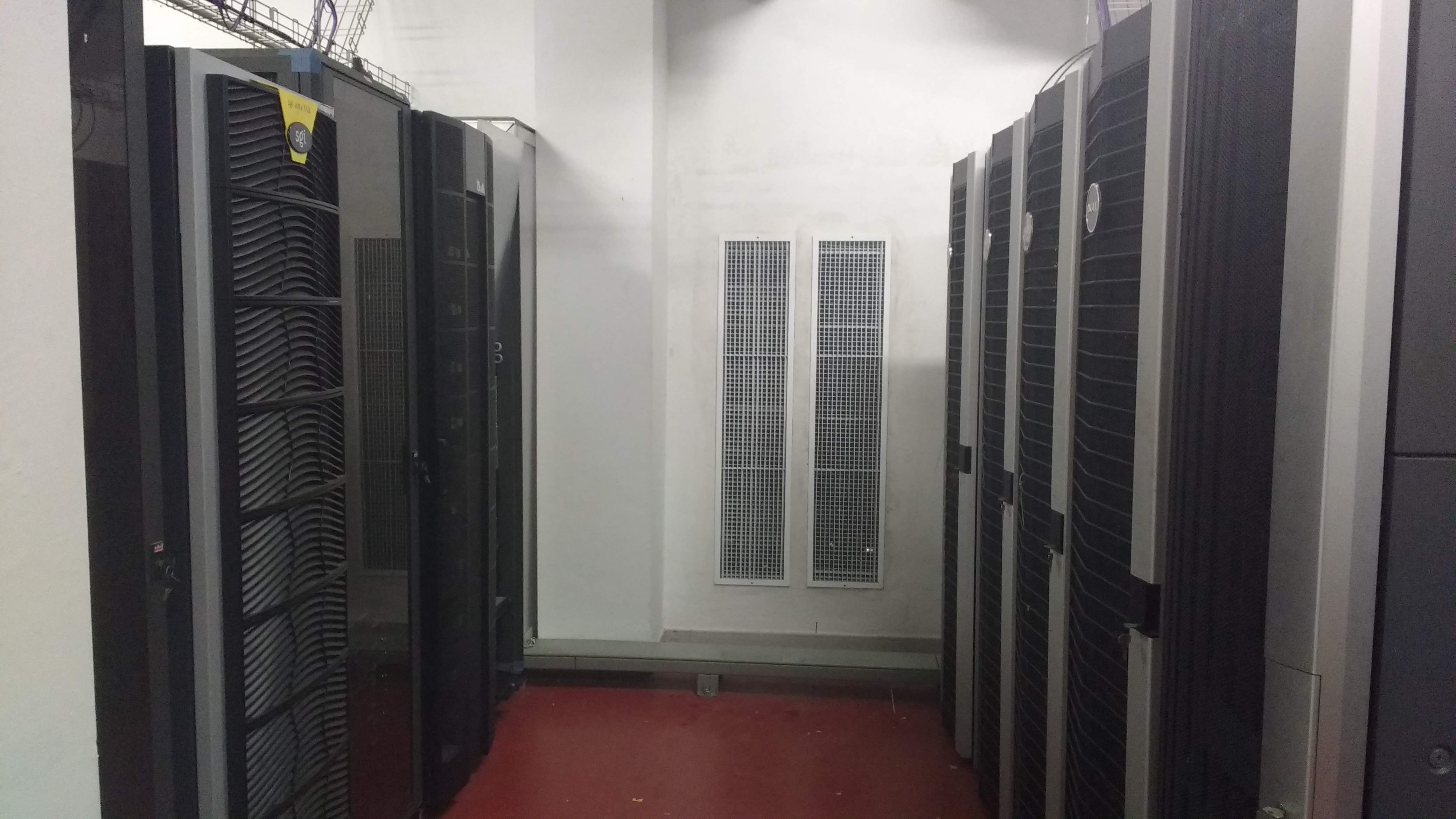
When I saw the supercomputers for the first time they were and are very special machines for me. They are very big with many nodes. They also need a lot of power. I often wonder how they can be so powerful, and how they can stay at a low operating temperature? Also they need to more power. How can they run more quickly ? How can they be cold? Actually these questions are asked with the question of “What is the HPC? ”
I was learning everything step by step. I have previously worked with super computers without seeing them, I just imagined them. After seeing them, absolutely yes, they are so incredible.
I met many cheerful people who work at CINECA. My site coordinator name is Massimiliano Guarrasi. He introduced me to everyone. He is also very helpful 🙂 My project mentor works in Bologna University so he is not be at CINECA every day. Up to now, we have defined my project progress. When I have a problem with the project we talk with my supervisor by email or skype. I work at CINECA but my project mentor is always with me and replies to my requests.
My project goal is to implement Web visualization of energy load in HPC systems. I use Grafana to visualize, and python to manage and implement the system. How can I do this ? What is the Grafana? What does the data look like when visualized? Which super computer do I use? I will explain all this in another post.
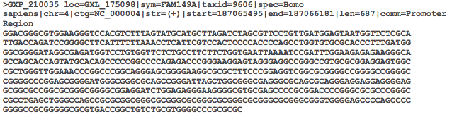
It has been a bit more than a month since my project began. Initially, the learning curve was rather steep as the project I am working on, ABySS, a bioinformatics software for assembling DNA sequences is complex and consists of many intertwined parts and processing stages. Still, as I got to explore its workings, at this point, there’s measureable progress.
Assembling genome is a long process and involves manipulating large amounts of DNA data, especially if the genome is long, as is the case with humans. As such, performance is of great importance, as you might be assembling the DNA multiple times (or of various species) and you only have so much time to do that. These jobs can last days, so even a seemingly unimportant performance boost can save you a day or two.
My first step was to determine the bottlenecks, parts of the code whose execution time directly impacts the execution time of the whole program. To quicken the process, I have contacted the original program creators at Canada’s Michael Smith Genome Sciences Centre. They were happy to quickly respond and point out possible improvements, as well as what I can investigate more into.
My first task was to improve an in-house DNA file reader. DNA is stored in FASTA or FASTQ file format, which is a text format holding nucleobase strings (A, C, T, G), along with optional DNA read quality, in FASTQ files. The main problem with the existing reader was that buffering was not done right and the reader was making more reads than necessary, and file reads are slow. What you ideally want to do is read files in big chunks and then process that in-memory. There is a library that does this for FASTA/FASTQ files called kseq, so my goal here was to integrate it with the existing reader. The integration was done in such a way that the original implementation persists, but the program will prefer to use the new library if possible (based on file content).
A FASTA file content.
After benchmarking the new file reader, I have found that it was twice as fast as the old one, so it was a success. However, that was only performance of reading single files without any processing whatsoever. Upon testing the whole program on real data, I have found that the performance improvement isn’t as much (up to 10% difference in wallclock time), but that was to be expected, as reading files is only a small part of the whole pipeline.
After this, I have moved on to see if I can make more significant speedups. Turns out, after profiling the execution, there is a particular data structure that slows down the process a lot. So called Bloom Filters, which are a probabilistic data structures for testing whether data exists in a set have to be constructed from DNA data. These filters are built directly from FASTA/FASTQ files and basically tell whether a particular DNA sequence exists in a set. As these filters are large, their build process is multithreaded in order to speed it up, but to make sure this process works correctly, each thread has to exclusively lock the part of the data structure it’s building, in order to prevent other threads from meddling. This causes contention between threads and a massive slow down, as threads have to wait one another to access different parts.
The solution? Lockless filters. Get rid of locks altogether (almost). Instead of having threads fight one another for access rights, what I have done is give each thread its own copy of the bloom filter to build and then merge them in the end. The speedup was very noticeable, and the process lasts half of what it did before. There is a catch, however, I have realized only later. The size of these filters varies from 500MB up to 40GB, and is a configurable parameter. If you are dealing with filters of size 40GB on a 128GB RAM node (which is the case at Salomon), you can not have more than 3 copies of the filter at a time. But it is possible to alleviate this problem, as you can specify how many threads should have their private copies of the lockless filter and the rest of the threads use a single filter with locks. This way, the more memory you have, the better the speed up, with a copy of the filter for every thread in ideal case with sufficient memory.
While I was doing all this work, I received an email from my mentor – I was to give a presentation about my progress to him and maybe a few other people. Sure, why not, this would be a good opportunity to sum it up for me, as well. Few days later, when I was about to present, I realized it was more than a few people! Most of the seats were filled and the IT4I Supercomputing Services director, Branislav Jansík himself came. The presentation lasted for about an hour and most of the people present had several questions, which was pretty cool, as they managed to understand the presentation, even though not all of them were in technical positions.
Giving a presentation on my work so far.
The presentation was a very useful experience though, as it was, in a way, practice for the final report. It was far from what a final report should look like in terms of quality, but thankfully, I have received a lot of feedback from my mentor that will help me get the final presentation right. So big thanks to Martin Mokrejš, who also took the photo above!
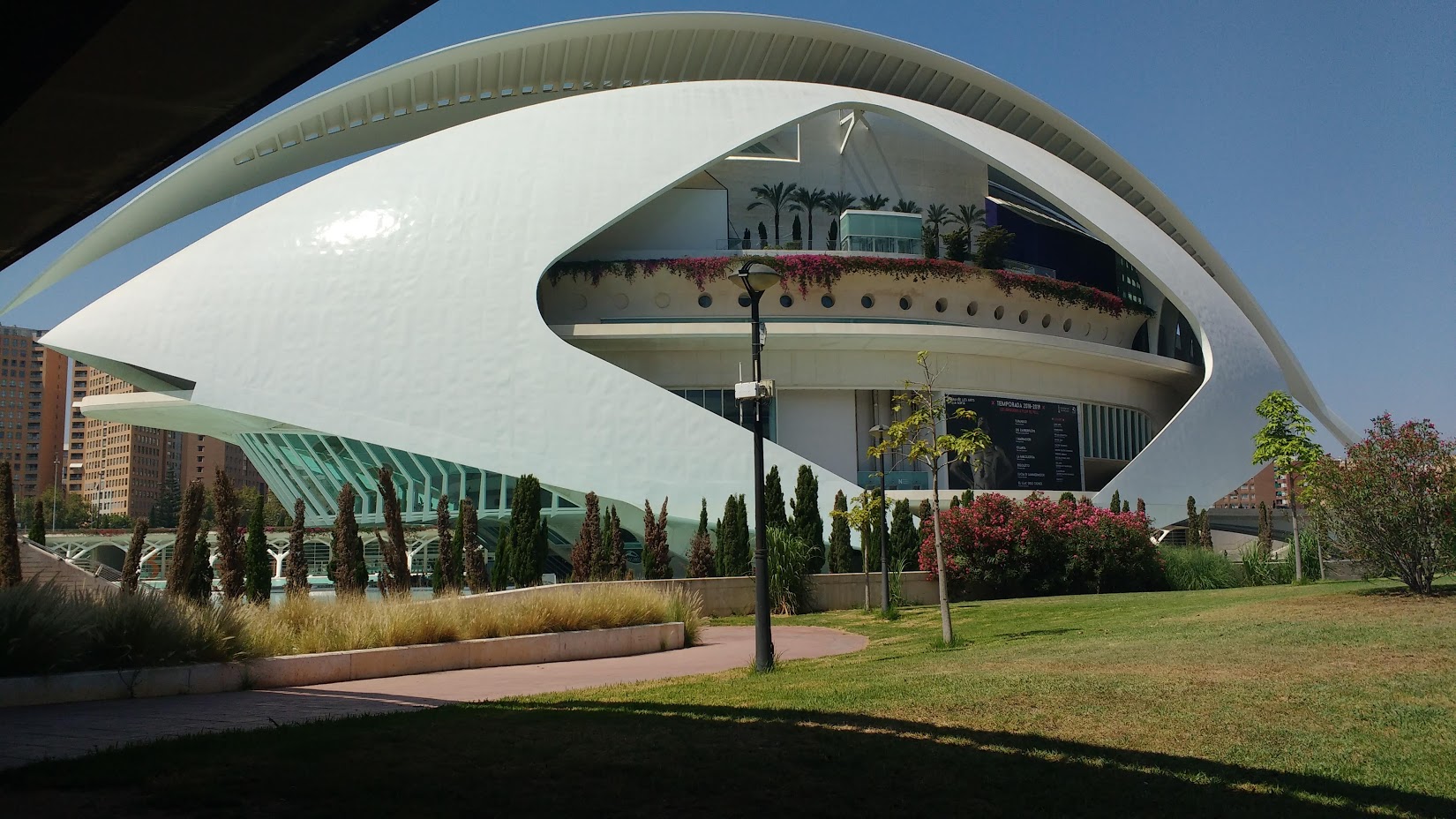
It’s been already 1 month here in Castello de la Plana, Spain for the PRACE Summer of HPC programme and one thing I have realized for sure is that the time passes really fast when you are having fun. But, what do I mean by fun? I will start explaining it by saying how I spend my weekends here. Trips to the towns next to Castello, for example Valencia, walk around the city and visiting the beach are some of the things I do after I finish work. It’s really relaxing.
Palau de les Arts Reina Sofia, Valencia.
But, SummerofHPC is not only about trips on weekends of course, but also working on interesting projects during the week. So, what is my project about ? It’s called ‘Dynamic management of resources simulator’ and I know that the title doesn’t say too much, that’s why for the rest of this blog post I will try to explain it.
Let’s decode the title. First, what does ‘management of resources’ mean? In HPC facilities, many applications can run concurrently and compete for the same resources. Because of this, ‘something’ has to boss around these applications by giving the resources to some applications while others are waiting. Here is where the resource manager (the ‘something’) kicks in. A program that has only one specific job, to distribute the resources to the applications based on a policy.
So far so good, now we can understand the part of the title which says ‘management of resources’. What about ‘Dynamic’? Something that is not obvious of course from the project’s title is that in this project we will deal with malleable applications, or let’s say better malleability. Malleability is nothing more than a characteristic that an application can have to change dynamically the number of its resources while it is running (on the fly). From this, we can see that an application can run with less resources by allowing more applications to run concurrently, increasing by this the global throughput. It makes sense now to have a resource manager which exploits malleability.
We have explained 80% of the title, the other 20% is the word ‘simulator’. Imagine that you want to run some applications on the HPC facility, what do you have to do ? First you have to login to the cluster, wait for the nodes to be freed (to allocate the nodes), then upload all the applications you want to run on the cluster and run them. Finally, pray to God that no-one interfered with your results. Too much effort. What about having the same behavior even on single-core machine (2018, hard to find a single-core…)? This is what the simulator is for. Let’s say that after this blog post, you get very interested in malleability and after some time you come up with an algorithm that exploits malleability. Will you try test your algorithm on the actual system? Well, of course you will do it at some point later, but first test it on the simulator without any cost.
To summarise, the purpose of this project is the introduction to the field of resource managers the concept of malleability by developing a simulator that executes a workload. By tuning different reconfiguration policies, we can determine the best configuration for fulfilling a given target without running the workload on an actual system. We are using Python and SimPy (simulation framework). We have implemented the simulator but right now we are in the phase of testing it. I am sorry that I don’t have any picture related to my project but I am writing code that I run it on my laptop, not even on an HPC system. On the other hand, since I am close to Valencia, I can share some paella…
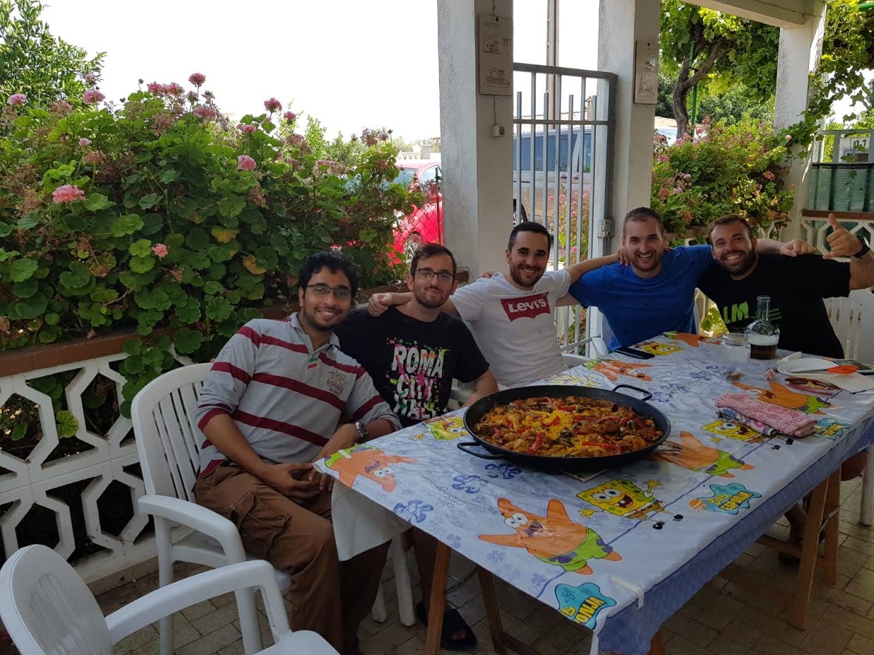
Me, Sukhminder, our supervisor, paella and the SpongeBob SquarePants tablecloth…


 Making friends abroad might often be a challenging task, however, it is easy if you play


 Hi from Bologna ! 🙂 It has been 5 weeks since I came to Bologna.