Hi there! If you are here it is probably because you read my previous blog posts or perhaps you are in search for a tutorial on how to calculate the thermal conductivity of a crystal… in any case you are in the right place, because in the following I will explain the simulations I performed for my Summer of HPC project ‘Computational atomic-scale modelling of materials for fusion reactors‘. To understand the context of these simulations I would highly suggest reading by previous blog post if you’re interested.

First of all we need to understand what thermal conductivity is. Usually expressed with the letter ‘k’ the thermal conductivity of a material is a measure of the ability of that material to conduct heat, and is defined by the Fourier’s law for heat conduction q=-k ∇T, where q is the heat flux and ∇T the temperature gradient.
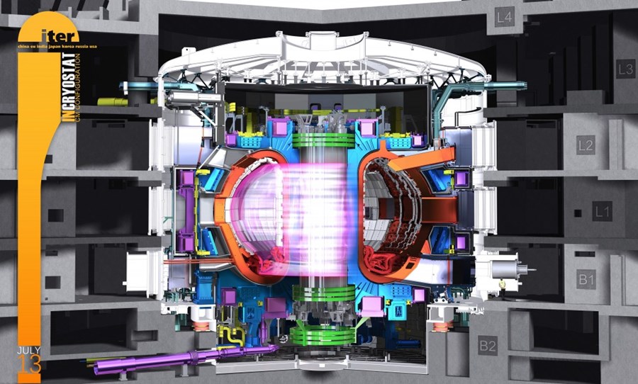
A material with an high thermal conductivity has an high efficiency in the conduction of heat, and that’s why it is important that a material like Tungsten has an high thermal conductivity for its application in a nuclear fusion reactor.

In this simple image the relation between the heat flux and the temperature difference at the two extremes of the solid is given by the thermal conductivity of the conducting solid.

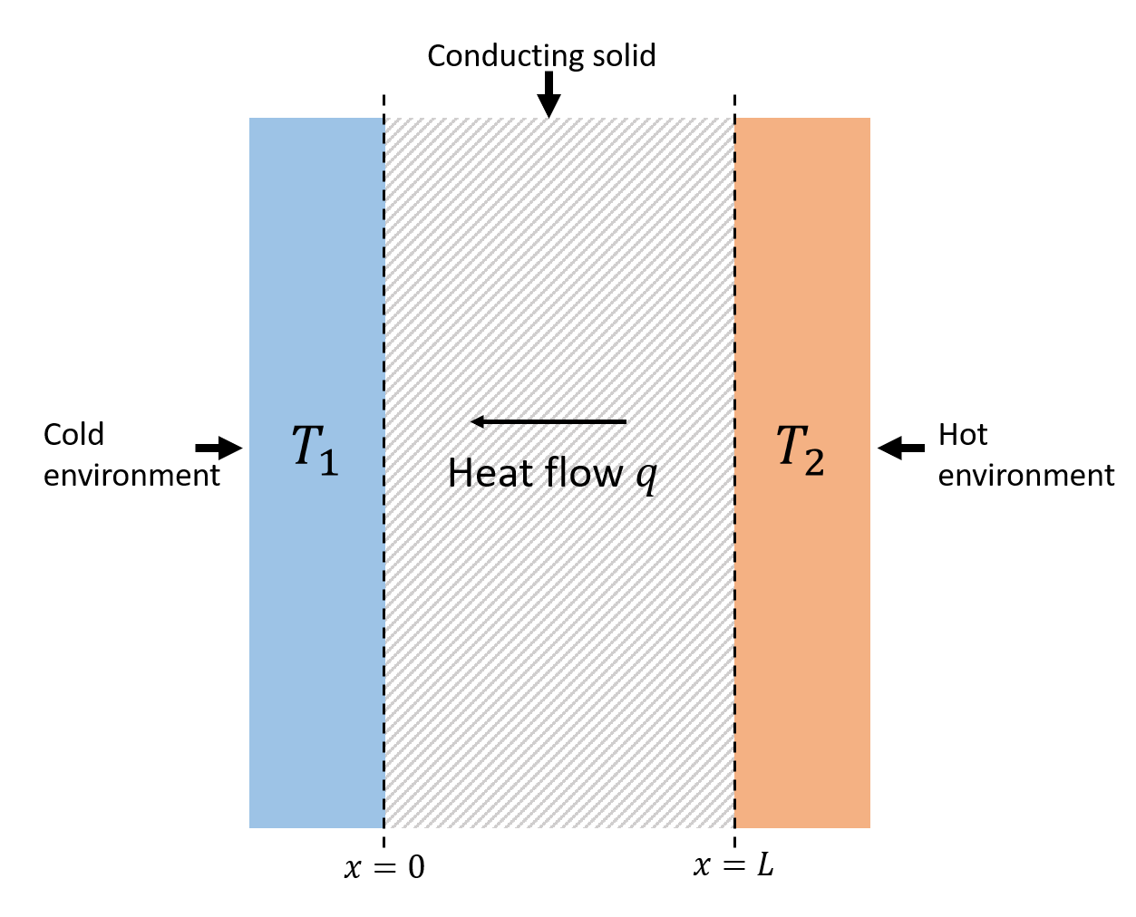
How can we calculate the thermal conductivity of a material? The relatively easiest way is to do it experimentally, applying an heat flux to the material and calculating the resulting temperature gradient; but this approach does not allow to investigate the effect of vacancies and defects at an atomic level, and that’s what we are interested in, since this defects while be formed by neutron bombardment.
And it’s here that molecular dynamics simulations come into place, with an atomistic simulations it is in fact possible to recreate this kind of configurations and investigate how they effect the thermal conductivity of the material. But first we need a reference value, so the the thermal conductivity of a perfect Tungsten crystal must be computed.

To do so in this project the LAMMPS code has been used, and the simulations have been performed on MareNostrum supercomputer of the Barcelona Supercomputing Center (BSC).
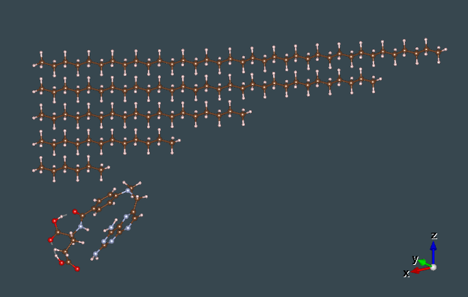
A parallelepiped simulation box is defined and Tungsten atoms are placed in a body centered cubic (BCC) crystalline structure, then an equilibration run is performed at a given system temperature, we used 300K to compare the results with previous papers. To have a constant temperature system LAMMPS uses a modified version of the equation of motion, the procedure goes under the name of Nose-Hoover algorithm.
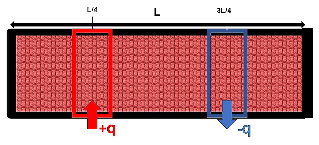
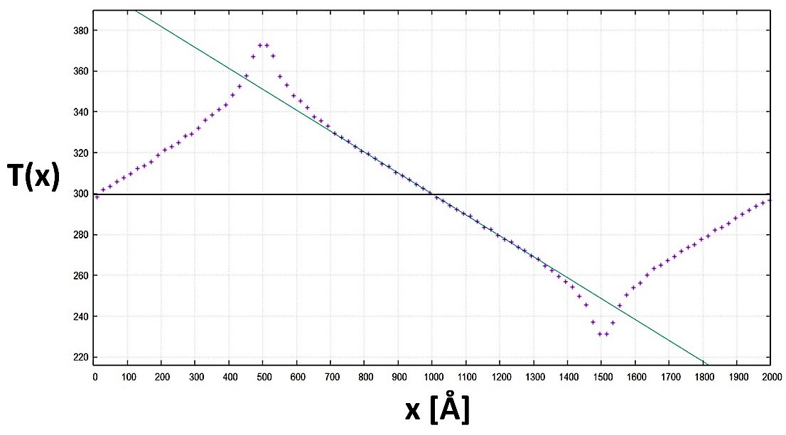
Once equilibrium is reached two regions are defined along one direction of the simulation box, at equal distance from the box borders and of equal volume, using an appropriate command a positive heat flux q starts heating one of the two regions, while an equal but negative heat flux q starts cooling the other one.

Scheme of the simulation box and the two, positive and negative, heat fluxes.


In this way the average temperature of the system stays constant, but the first region will locally have an higher temperature while the second one a lower one, we then have a temperature gradient ∇T between these two regions; knowing the value of the heat flux q and calculating ∇T we obtain the value for the thermal conductivity k from the Fourier’s law.
This procedure has been performed using different potentials and system sizes obtaining results agreeing with previous papers.

Example of a temperature profile of a system of tungsten atoms. The black is the average temperature, while the green one is a fit of the central region from which the temperature gradient is obtained.

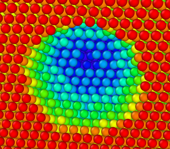
We then proceeded to add an empty bubble at the center of the system with radius r, resembling the damage caused by neutron bombardment, and repeated the same procedure obtaining a new result for the thermal conductivity of the system.
We investigated the relative variation of the thermal conductivity with respect to the value for a perfect crystal increasing the size of the empty sphere at the box center; the obtained result is a decreasing linear behaviour of the thermal conductivity as a function of the transverse (with respect to the heat flux direction) area of the sphere πr2 ; the result is shown in the following graph. For high radius spheres we start to see the effect of the finite size of the simulation box, which is not infinite, and the behaviour shifts away from the linear one.

Variation of the thermal conductivity, with respect to the perfect crystal value, as a function of the empty sphere cross area relative to the simulation box cross area.

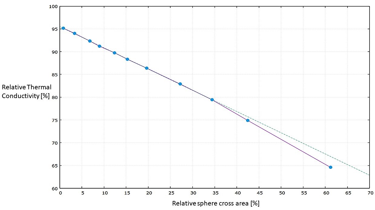
These vacancies have an important effect on a crystal system like this one, to give you an idea the first point of the graph corresponds to the removal of 11 atoms from an half million atoms system, and the thermal conductivity already drops by 5%; this is the same reason why it is so crucial to study and understand the effect that these vacancies cause on a system, since these structures will be formed also in real life conditions with real effects.
The results obtained in this project can be used as a basis to further explore this type of defects, for example injecting inside the empty bubbles Hydrogen or Helium atoms, resembling what really happens when this atoms escape from the nuclear fusion reactor core.


I’m really grateful to every person that made my partecipation for the Summer of HPC 2021 possible, it has been a wonderful experience, learning new computational skills and techniques and meeting amazing people; it is a fantastic experience that I would recommend to anyone interested in computational science and its applications.
I hope you found my blog pages interesting and helpful, if so you will sure like the posts my colleague Eoin did on the formation of defect cascades. Have a wonderful day!

Hello people! Bartu from project 2128 here. This summer, I was responsible with the development of a reliable software to generate spur gear pairs. First, let me tell you about the procedure we follow for gear generation.

The Procedure

To generate a gear, we first need to calculate some points that will create the necessary curves once interpolated. For this, we use the equation of basic rack profile for spur gears to obtain the addendum part of the gear. After that, we calculate the points that are on the pitch circle and that will connect the pitch circle body of the gear to the gear teeth. These calculated points are then checked for validity and rearranged if they are good to proceed with the drawing part of the procedure. Later, straight lines are drawn between the calculated points to join them together and obtain a completed gear profile on a 2D plane. This profile is then extruded by the user specified amount, thus generating a 3D gear model. The same procedure is repeated for the second gear, which will complete the gear pair. The second gear is then translated in 2D into the correct orientation for analysis, producing the geometry shown below.

The Generated Gear Pair

Important Considerations

We have decided to separate the process into two to allow parallelization and error handling, being more reliable for the user and easy to develop further for the developer. This way, all of the point calculations and validation checks are done in parallel outside our drawing software SALOME, essentially making it impossible for SALOME to crash. The procedure failing inside SALOME can be a real waste of time so we focused on eliminating that.

Hi stranger on the internet! If you clicked on this webpage you’re probably interested in material science, or maybe you were just intrigued by the title, or perhaps you just misclicked…
Anyway, in the following I will briefly explain how my project ‘Computational atomic-scale modelling of materials for fusion reactors’ is structured and what are my objectives, so feel free to check it out if you’re interested.

You probably heard before in a way or another about nuclear fusion, it’s the main process that happens inside our Sun, and all the other stars, and generates the energy that makes life possible here on Earth.
Today different projects involving the world most powerful countries are trying to reproduce nuclear fusion on earth and make it a new source of energy, possibly changing forever our energy production methods.
In the context of this nuclear fusion reactors different branches of physics, chemistry and engineering come together to achieve this incredibly difficult task, but that could lead to one of the greatest achievement of mankind; one of these branches is material science. Specific materials must be used in a nuclear fusion reactor, that can sustain the incredibly harsh conditions present; to give an example ITER is currently the largest experiment of nuclear fusion under construction and at its core it will reach temperatures of around 150 million degrees, ten times higher than the temperature of the core of the Sun!

Concept image of the ITER nuclear fusion reactor

Source: ITER official web page https://www.iter.org/proj/inafewlines

One of the materials that is used in a nuclear fusion reactor is Tungsten, due to its high thermal conductivity and highest melting point of all metals. Which makes it perfect for the harsh conditions it is subject to, but it faces a critical problem: the damage caused by the particles present in the fusion reactor: the two hydrogen isotopes, deuterium and tritium, which are the input particles of the fusion reaction, helium atoms and neutrons which are the products of the reaction alongside energy.
Some of these particles can in fact hit the material causing damage at an atomic level because of their high energy, given the temperature of the core. For example neutrons can initiate chain events from an initial collision with a tungsten atom, which are called defect cascades, that will result in the displacement of several atoms from the lattice structure and the formation of vacancies.

This changes in the structure will then affect the properties of the material, and such variation need to be studied to have a clear picture of what will happen in nuclear fusion experiments like ITER.
While the work of my colleague Eoin was focused on reproducing cascades of defects inside tungsten; mine was centered around the thermal conductivity of tungsten and in particular the effect of defects on such property, like the presence of large vacancies, which can be also filled by Hydrogen and Helium atoms.To do so molecular dynamic simulations, using the LAMMPS code, have been performed. The basic idea of molecular dynamics is to create a system in which single atoms are present and each one evolves in time using the classical Newton’s law of motion and a potential that is given depending of the material of interest. Millions of atoms can be simulated using such simulations, and even if quantum effects are not considered, the great number of particles, which could not be possible in a quantum simulation, allows to study very well properties like thermal conductivity.

Example of an empty bubble inside a Tungsten atoms system in a molecular dynamics simulation. Structures of this kind will change the material properties!


(the colouring of the image is used to give a sense of depth)

If you are interested in the topic you can give a look at my next blog post, which will be focused on a procedure to calculate the thermal conductivity of a crystal using molecular dynamics and my results with Tungsten.
If the idea of the defects cascades has caught your attention my colleague Eoin has written some blog posts on the topic on his page.
In any case, thanks for your attention and I hope you enjoyed this blog post. Have a good day, dear internet stranger!

Hi! So, this is a bit awkward. To be honest, I kinda forgot about these blog posts, and whenever I remembered I was already too busy with something else and ended up forgetting again. So finally, here we go:

Hello! I’m Andraž, a Computer and Information Science student at the University of Ljubljana in Slovenia. Conveniently that’s also where I’m from, so I never had to go far to attend uni. I’ve been interested in HPC for a while and have done some student work in the field, so this seemed like the perfect opportunity to get even more familiar with the topic and get a more genuine hands-on experience.

As a computer science student my interest was always more in the background/administration side of things when it comes to HPC, so a project like the one I ended up with (High Throughput HEP Data Processing at HPC – 2110) seems like the perfect fit for me, since it deals more with understanding how a cluster works and what its limitations are, rather than only using it for various computations. But I do admit I’m a bit disappointed about not having been able to visit the project site. Two months at CERN while working on this would have been fantastic! Alas, such is the world these days, it’s out of anyone’s control. (Well, not entirely: get vaccinated!!)

A bit more about me though, since this is meant to introduce me at least to some extent! At university I studied chemistry at first, until I realised I should probably have gone for computer science in the first place instead. Some time was lost, but a lot of things were learned! (I suppose that means no time was really lost, to be fair.) So I do have an easier time understanding some of the chemistry and physics behind the work I currently do, which is helping out with adjusting some software for molecular modeling at the National Institute of Chemistry. Aside from that I busy myself with fairly standard nerdy things: playing the piano, video games, series, films, etc. One of my recent interests has been diving into weird musical theory videos on YouTube, and I highly recommend anyone with an inkling of interest in it to try it out!

I think that’ll do for now, there’s only so much I can tell about myself before I start feeling weird about it. (Just talking about yourself while not getting to know someone else at the same time is a bit of a weird thing isn’t it?) Can’t wait to see what this project holds in store for me! (I suppose I already know since I’m so late with this, don’t call me out like that. I need to build some suspense at least!)

Greetings all,

Welcome back to my third and final blog post for the Summer of HPC. This is the final week of SoHPC and between the presentations and the report writing, I decided to write my final blog post to explain my work in more depth. In the previous blog post, I explained what fault tolerance is and why it is essential. Also, I introduced the FTI library and mentioned lossy compression as a technique to limit the IO bottleneck. In this blog post, I will explain more extensively the implementation of lossy compression in the FTI, the results of the until now experiments, and my future expectations. If you haven’t, I suggest reading my previous blog post so that you can understand the basic concepts of the FTI library in which the implementation was made.

Implementation

To execute FTI one must specify certain parameters in the configuration file (configuration example). To use the lossy compression feature, three extra parameters must be specified: compression_enabled, cpc_block_size, and cpc_tolerance. The first one is simply a boolean value which, when set to 1, allows the checkpoints to be compressed. The second one specifies the maximum memory size which can be allocated for the compression and is used to protect memory restricted systems. It is suggested that the block size is not significantly lower than the actual data size, because then it will interfere with the compression and may decrease the compression ratio. The last parameter defines the absolute error tolerance for the compression. The actual error tolerance is given by the function 10-t where t is the integer cpc_tolerance specified at the configuration file. The user must specify a tolerance suited for their application, high enough to maximize the compression rate, but low enough so the results won’t be altered.

Experiments

Ckpt size as a function of tolerance
Figure 1: In this graph, we can see the size of the checkpoint file of rank zero for different tolerances in comparison with the checkpoint size without compression.
Ckpt write time as a function of tolerance
In this graph, we can see the write time of the checkpoints for different tolerances in comparison with the checkpoint write time without compression.

As a principle, lossy compression targets large-scale applications. Although the performance of lossy compression differs for different data sets, in programs with small memory, using lossy compression may even slow down checkpointing due to the time needed to perform the compression and the possibility of hard to compress data. Therefore, to test the application we have to employ a very scalable application. For our experiments, we run LULESH on BSC’s Marenostrum cluster, with a size of 615,85 Megabytes per process, for 512 processes in 16 different nodes, using different values for cpc_tolerance. The experiment can be considered successful since a measurable decrease in the time to write the checkpoint was observed. As you can see in figures 1 and 2, the write times of the checkpoints for any value of tolerance between zero and eight seem to be around half the write time when the checkpoint isn’t compressed. Also, we can see that tolerance doesn’t really affect write time, since for different tolerances we don’t observe high differences at the checkpoint file. This may change in other experiments with different data consistency or size.

Video Presentation

For the closing meeting of SoHPC, my partner Kevser and I created a five minute video presentation explaining our project.

Project video presentation

Finally

That summarizes our work in the SoHPC, I hope you found it interesting. As this experience comes to an end I would like to express my gratitude to the organizers and project supervisors of SoHPC for the great work they are doing. During the summer I learned a whole lot of new things, gained experience in working as a researcher, and collaborated with many inspiring people. Finally, I undoubtedly encourage every student interested in HPC, and computing in general, to apply to SoHPC because it is a very positive and unforgettable experience, which I am grateful that I had during my studies.

Hello everyone, my name is Spyridon-Andreas Siskos and my friends call me Andreas. I am 25 years old and I am studying Computer Science at the University of Crete. My main interests are in computer networks, security, and algorithms. I really like to solve problems in networks and security and finding the most optimum way to do it. In my free time, I like to spend time with my friends, going out and see new places and playing together sports like football, basketball, and many others!

One day, a professor from my department sent us an e-mail talking about a very interesting summer internship in high-performance computing. When I saw it, I really liked a project called “Quantum Algorithms and their Applications” from its description, because it was talking about quantum algorithms that I didn’t know a lot of things about them and I really liked two of them.. Shor’s and Grover’s algorithm. I was so excited about it and I immediately checked how to apply for it! There was a very interesting algorithmic challenge in order to get into this internship and I liked that a lot too!

Then, I got accepted into this summer internship and I was so excited about it! Now, I have learned a lot of things about quantum computers and their algorithms, I have implemented some of them, but this was not only the good part of this internship. I also worked with Lucía, a very good and intelligent girl that helped me a lot in understanding a lot of things about quantum computers and the maths behind them, and we had a lot of fun when we were working on our project!

Greetings everyone!

Welcome to my second post about my experience with Summer of High Performance Computing. First of all I hope that you are doing well and you had an enjoyable summer. If you haven’t already, go check my previews post, so you can get to know me a little better.

Hartree-Fock Algorithm

As I mention on my previous post, this summer I was working together with Eduard Zsurka under RNDr. Ján Simunek guidance, in order to implement and test a BLAS (Basic Linear Algebra Subprograms) version written in Fortran, to an existing code of Hartree-Fock algorithm written by Ján Simunek et al. What is Hartree-Fock you may ask. Simply put Hartree-Fock is a method that it can give us an approximation for the determination of the wave function and energy of a quantum N-body system in its ground state. Even simplier put, what this method does is to do an approximation solution of Schrödinger equation.

In this method there are two time consuming steps in the algorithm. One is the formation of Fock matrix which is a approximation through iterations to the single-electron energy operator for a given basis set and derives from integrals and density matrix. The second step is the diagonalization of the Fock matrix, which for linearly scaling methods and parallelization is an unwanted step. Dr Simunek et al. managed to replace the diagonalization step by replacing it with matrix-matrix multiplications. For larger molecules the electron integral matrices are sparse. Sparse matrices have the advantage that only the non-zero elements need to been stored and thus the matrices are occupying less memory.

Our task was to find libraries that can handle sparse matrix multiplications written in Fortran. The first two candidates where two libraries, one from National Institute of Standards and Technology (NIST) and the second one from netlib. With both of these libraries we had difficulty to successfully implement them to existing code, because of lacking documentation or not compiling with newer versions of Fortran. By that time we were searching for another way to implement from those libraries a sparse matrix-matrix multiplication or even to use intel’s Sparse BLAS library, we found a stackoverflow post with a guide for a working implemantation of netlib’s library.

5 Alkanes and Methotrexate used as testing molecules.

After we managed to have a working test code from the said library we tested to methane molecule, where we found that our test code was working. Succeeding that we started testing the code on methotrexate (C20H22N8O5), and 5 different alkanes: C6H14, C12H26,  C18H38,  C24H50, C30H62, C36H74. Starting with methotrexate the results weren’t that great since our code was actually slower than the original code. These results didn’t disappoint us at all since we knew we had to go for bigger molecules, where we have even bigger sparse matrices.

This is the end of this post. We managed to have a working code and we are looking forward for more results. In my next post, we are going to see if for bigger molecules we can decrease the running time of the code. Thank you for reading my post.

In a repository far, far away, Stan is being developed.

The struggle for efficient sampling

“It is a period of computational war. Random walkers, striking from an initial position, have sampled from probability distributions and computed their first expectation against the continuous Random Variable. During the sampling, the Statistical Community managed to steal secret measure-theoretic descriptions of the Distribution’s ultimate core, the typical set, a singular portion of spaces with enough density-volume tension to compute an entire expectation.

Plagued by the Curse of Dimensionality, Morten and I race home aboard HPC, to implement the secret code that can save our fellow data scientists’ time and resources and sample efficiently in the galaxy.”

Low-performance cats, a constant negative example for the project.

Welcome back! Last time I left you with a general introduction to the project and HPC. Now let us dive into some details!

Stan and MCMC

Stan’s a framework “for statistical modeling and high-performance statistical computation”, as the official page states, and is used extensively by statisticians and scientists. Among other things, it offers algorithms for Bayesian statistical inference: it is the use of data analysis for determining the properties and the parameters of a probability distribution, using the Bayes’ theorem. Now, if the probabilistic model can be expressed as a graph, where a node represents a random variable (RV) and an edge the conditional dependence between RVs, then we can use simulation algorithms, like Markov Chain Monte Carlo (MCMC) methods. The idea is pretty simple: these algorithms sample from RVs, using those samples to compute integrals over that RV, such as expectation or variance. How do they sample? An ensemble of random walkers wanders around the space, applying the so-called Markov transitions and trying to obtain samples that will contribute significantly to the integral.

Logo of the statistical framework we have been using and trying to contribute to.

As you may imagine, lots of MCMC algorithms exist, with their ups and – especially – downs. Simplifying a bit, they can waste a lot of computational resources (and time!) sampling from regions that are irrelevant for computing those integrals: the integrals make use of both the distribution and the volume, and it turns out that, while the former is mostly found near the mode, the latter quickly accumulates away from it. Only a very narrow region, more and mo\re singular as the dimension grows, contributes to the integral: the typical set. How to reach and explore it? An ingenious method called Hamiltonian Monte Carlo (HMC) has been devised that simulates Hamiltonian dynamics, treats samples like physical particles, and exploits the symplectic properties of the Hamiltonian flux to approach and explore the typical set efficiently.

Wanting a better HMC

Now, Stan offers some great MCMC algorithms, and HMC is among them. Our job for this project consisted in implementing a yet more efficient version of the HMC and, if possible, parallelise it!

One thing about HMC is that it doubles the space dimension and has two variables to handle: a position and a momentum. The momentum allows a particle (~ sample) to follow the field lines and us to exploit the gradient of the distribution to direct it properly. How, you may ask? As with any numerical simulation, we need to integrate the orbit, and do so with the symplectic integrators, which have the nice property of volume preservation: this means that the computed path cannot deviate too much from the actual path, even for long integration times. Symplectic integrators can be derived from the Hamilton equations and can be of any order k; the simplest ones being:

  • k = 1: symplectic Euler
  • k = 2: Störmer-Verlet, with variations (such as the leap-frog, which we used!)
The kick-drift-kick scheme used by the leapfrog integrator.

The HMC, after every integration, obtains a proposal and decides whether to accept or reject it, i.e. to keep it as a new sample or ignore it. To do so, it computes the total energy (or Hamiltonian) of the system before and after integrating: samples whose energy has reduced in the process are accepted unconditionally, while the others are exponentially more likely to be rejected.

Building a better HMC

We were given a very complex C++ code skeleton to be completed and/or reformatted; this code could be submitted to the Stan Framework. The way we proceeded is as follows:

  • we implemented a data structure using the Structure of Array (SoA) model: the ensemble of particles holds one array for each particle’s feature (so 2 arrays in our case: positions and momenta);
  • we completed the integrator structure, devising how the integration should be performed: namely, with the afore-mentioned leapfrog;
  • we added functionalities to another script for the actual computations: in there, the algorithm samples, computes the Hamiltonian, and decides if to accept or reject the proposals; finally, it estimates the parameter of the input model (after all, we’re performing what is called stochastic parameter fitting).

We are pretty satisfied with our implementation since it’s fast and produces meaningful results. Still, there’s a world to be explored!

Beyond HMC

For example: when implementing the integration, we had to specify a step size and a number of steps, since these are not automatically computed by the algorithm. We have also experimented with a 3° order “Ruth” integrator, which turned out fast (and required a larger step size and a smaller number of steps). There is a variant of the HMC algorithm, the No-U-Turn Sampler (NUTS), which eliminates the need for setting the number of steps (and offers some heuristics for computing a good step size).

But that’s for another time! Thanks for your attention.

Navier-Stokes equations are a set of PDEs not analytically solved. They are one of the unsolved mathematical problems of the Millenium, which resolution will give the award from the Clay Mathematics Institute. However, they completely describe the fluid’s behavior in all situations. Navier-Stokes equations are a system of three laws of equilibrium: mass, momentum, and energy. The first one is also called the equation of continuity, the second corresponds to the First Newton’s Law, while the last one is the First principle of Thermodynamics. They can be written in different forms, referring to a finite control volume (integral form) or an infinitesimal control volume (differential form). In addition, this control volume can be considered fixed in space and time (Eulerian approach, conservative form) or moving with the fluid (Lagrangian point of view, non-conservative form).

Incompressible Navier-Stokes equations. d is the dimension of the problem, i.e. one-dimensional problems d=1, bidimensional problems d=2, three-dimensional problems d=3.

To understand and analyze the behavior of the external or internal fluid flow, we have two different possibilities: experimental investigation or numerical approach. The first one was the most used in the first years of studies when computer architectures were not so advanced. Nowadays, with the usage of the HPC systems, the numerical approach is becoming the most important. In this context, the CFD is placed. Computational Fluid Dynamics uses numerical techniques to discretize the Navier-Stokes equations. In other words, with the CFD, we are searching for the solution at a specific point, which depends on the typical numerical method that we are using, then, we reconstruct the solution somewhere else with a technique that, again, depends on the numerical method selected. There are a lot of numerical methods: finite difference, finite elements, finite volume, spectral methods, characteristic lines, hybrid discontinuous Galerkin method, etc. All these methods use the same already explained idea. All these are already implemented in different solvers. The one that we are using is the free open-source OpenFOAM.

The usage of the HPC system in fluid dynamics has become interesting with the studies of turbulent flows. Turbulence is described by the Navier-Stokes equations and it is a regime of fluid motion. Even if there is not a specific definition of the turbulent regime, we can describe it as a flow with three-dimensional, unsteady, and non-linearly interacting vorticity.

Effect of the shape on the drag aerodynamics of the car. Sketching of vortices and turbulence in the wakes. The picture was taken from https://www.reddit.com/r/Design/comments/krgg3o/advertisement_from_the_1930s_showing_the_advanced/

Modeling the turbulence, several methods are present in the literature. Generally speaking, the main attention must be focused on which details we want to analyze. An increment in this will introduce an increment in the computational cost. For these reasons, the DNS is not used in the industries. In general, they reach a maximum the LES, even if in the last period most of them are considering the DES. Let’s describe these from the bottom to the top:

Turbulence modeling
  • RANS: it is the acronym for Reynolds Average Navier-Stokes equations. With this strategy, we are decomposing the entire flow field as a sum of two different contributions: the first one is constant in time and it is associated with the mean flow. The second one, instead, is time-dependent and is associated with fluctuations. Using this decomposition for all the quantities present in the equations (velocity, density, pressure, etc.) we can see that in the momentum equation a new term appears. It is similar to stress and, for this reason, is called Reynolds’ stress. This term needs to be modeled. Hence, new equations must be added. Many numerical methods try to close the system. The classical numerical method based on one equation is the Spalart-Allmaras, while based on two equations there are the k-Epsilon, k-Omega, and k-Omega SST. URANS stands for Unsteady RANS.
  • DES: it stands for Detached Eddy simulation. It is a hybrid technique that considers both the RANS and the LES approach. The idea of the DES is to reduce the computational cost of the LES but increasing the description of the RANS. It fixes a turbulent length based on the TKE and the turbulent dissipation rate. Then it compares the turbulent length with the mesh size: if the mesh size is lower than the turbulent length means that we are far from the wall, so we are interested in solving all the detached eddies, i.e. LES in applied. Instead, if the mesh size is greater than the turbulent length means that we are near the wall, thus no detached eddies are present, i.e. RANS is used.
  • LES: in the Large Eddy Simulations, we are interested in solving all the large eddies, without any approximation. Then, for the subgrid contribution, we need to introduce a model. One of the most important scientists that gave a big contribution to the LES was Massimo Germano, from my home University, and Smagorinsky.
  • DNS: the Direct Numerical Simulation solves all the scales, from the integral scales to the Kolmogorov scales, where the dissipation will take place. No approximation is needed, but we need to consider an increment in the computational cost. In these problems, nowadays, DNS is only used for academic works with simplified geometry, to understand the behavior of the turbulent flow under particular conditions.

In our project, we focused our attention on the RANS approach with different turbulence models: Spalart-Allmaras, k-Omega, k-Omega SST, and k-Epsilon. We use the OpenFOAM solver, which is based on finite volume discretization.

Streamlines and coefficient of pressure. You can see our final report for more detailed numerical results.

In the picture, you can see the Q-criterion applied for the three different geometries (fastback, estateback, and notchback) of the DrivAer, all without wheels following our Supervisor’s suggestion to reduce the complexity of the simulations. The simulations were running for 10 m/s inlet velocity, zero pressure gradient in the outlet region, k-Omega SST turbulence model, and for steady-states. The Q-criterion and the vorticity were computed directly on Paraview. It is simple to notice that the three different geometries provide three different turbulent structures in the wake. Obviously, big wakes mean big drag, i.e. higher request of fuel. Hence, more pollution.

Q-criterion. You can see our final report for more detailed numerical results.

As I come to the end of my time with IT4Innovations and PRACE, I have been reflecting on the amazing experience that I’ve had over the past eight weeks. Although I was not able to travel to the IT4Innovations National Supercomputing site in Ostrava, Czech Republic; I have had so much fun with my mentors and fellow interns online!

PRACE Timeline 2021 (Project 2118 specific)

Having the opportunity to work in a field that I love and appreciate has taught me so much. Below are a few key points that I have taken away with me after working in the quantum field for two months.

1. Ask loads of questions

Quantum computing isn’t the easiest of concepts to understand, and when I started my internship a lot of information went straight over my head. However, my mentor and colleagues encouraged me to be inquisitive and ask questions, no matter how silly I thought they were! This allowed me to solidify my understanding of quantum techniques and their applications to chemistry.

2. Take breaks little and often

A lot of the work I did during my summer involved coding in Qiskit, which can be intense and frustrating at times, especially when the code keeps breaking and throwing errors. I found myself staring at my computer screen for hours, and not getting anywhere with finding a solution. I started taking small breaks, so that when I came back to my computer, I could approach the problem with fresh eyes and a different perspective. Most of the time, I found the error almost instantly!

3. Draw diagrams

In a field like quantum computing and chemistry, where the concepts are so abstract, it can be hard to visualise the problem at hand. For example, in our project we were looking at the roto-vibrational dynamics of a hydrogen molecule, which is something we cannot physically see with the naked eye. To help with this, I found that sketching the molecules and interactions aided me with my understanding of core concepts, as I could picture what was happening at the subatomic scale.

4. Take every opportunity that you can!

With quantum computing being such a hot topic nowadays, it is important to gain as much insight and understanding you can, if it is something you want to be involved in. I have learnt to take every opportunity that I can, to get more experience in this exciting field, and ultimately contribute to the quantum revolution that we’re living in. Even if this means applying to a programme or job role that seems far out of reach – it’s always worth it! The probability that I would get accepted onto the PRACE SoHPC programme seemed slim, considering I did not have much previous experience in quantum. However, I showed my enthusiasm for the subject and I couldn’t be happier that I applied.

So, that’s all from me this summer. I can’t express how grateful I am to have had this opportunity, and I can’t wait to keep learning about quantum computing, and its applications to chemistry!

Here we are, we have arrived: these are the last days together of this fantastic adventure that was the Prace. I can’t believe it’s finished already, it seems to me yesterday that I was in my room following the week of traing! It was all so fast … but all so intense and wonderful.

I didn’t think I would learn so much, from familiarity with Python, to modifying and using programs for calculating VQE energies on IBM computers. I didn’t think I could write code for simulations … and what simulations! Seeing the molecules come to life in front of my eyes for the first time, because Jenay and I were able to make them do it, was a unique emotion that I will always remember. I remember that at first I was so scared, but then everything turned out to be easy to do, thanks to so much effort, study, passion, so much perseverance and tenacity!

A quick look at one of the codes used for the calculation of VQE energies
IBM Quantum Composer with the devices used for our calculations

Our mentors were fundamental: they helped, stimulated, followed and guided us all the time, giving us confidence and reassurance every moment.

So what does Prace leave me? Greater self-confidence, a lot of passion discovered for this field of work, greater confidence with programming, and a lot of gratitude for the people I met!

Thank you very much IT4Innovations National Supercomputing Center at VSB – Technical University of Ostrava for allowing me to work with them, and for their trust! I hope to visit the center in person someday.

Is it an experience that I recommend doing? Absolutely yes. And I already miss it so much …
I hope to get to know my colleague and my mentors in person, and maybe who knows, collaborate with them again.

Now let’s focus on the latest project work: our final report! And whatever happens, it’s a job that all of us at Project 2118 are proud of.

So there we are, that’s it for now. I greet my latest blog post with the great hope that it won’t be the last time!

Thanks Prace Summer of HPC

Hello there, I hope you’re ready to enter into the practical implications of our theoretical algorithm we saw last time. To refresh your mind, we want to find an elimination order of a graph that leads to lowest tree-width. To do so, our program will search a node separator using the flow-cutter algorithm with random inputs then cut the graph in several parts and repeat the process on sub-graphs until they are complete or tree. In practice, the flow-cutter algorithm is called multiple time, with random inputs, to extract the best possible separator and not just once which is too random. In order to manage the number of calls to the core flow-cutter algorithm, we use a parameter named nsample .Its default value is set to 20. Those calls are independent if we manage to work on several copies of our graph instead of references only. In this case, we would face some side effect with vertices and edges created and removed. Therefore, we can completely parallelize this section of code to gain computation time. To implement parallelism in Julia, we have several options but according to my lectures, there are mainly two of them:

  • Use threads with the Threads.@threads macro to parallelize the loop containing the sampling of input, the call to flow-cutter , etc.
  • Use coroutines/tasks with asyncmap-like functions to parallelize the calls to flow-cutter with known inputs

I’ve done some tests to compare both methods. I’ve run the two versions of the whole algorithm 20 times on the Sycamore 53 20 graph and I measured the average execution time with different numbers of threads. But quickly I saw that sadly the second method isn’t relevant for what we want to do. Indeed after a quick test I realize that asyncmap isn’t using multi-threads and thus does not speed up anything when its ntasks parameter varies. The resolution time is always almost the same as the single threaded version of the code. First I though that my code was wrong and this behavior came from mistake of mince but later I read more closely the Julia documentation and I noticed this little note in the end which says “Currently, all tasks in Julia are executed in a single OS thread co-operatively. Consequently, asyncmap is beneficial only when the mapping function involves any I/O – disk, network, remote worker invocation, etc.”. So indeed co-routines will not help us (today), but does threads ?

Running time of the whole algorithm on 1 node of Kay 40 cores
Speed-up of the whole algorithm on 1 node of Kay 40 cores

From this little experiment we can deduce that for the usual 20 calls to flow-cutter it’s better to use 9 threads to minimize the run time. Now we can write an MPI version of a wrapper which will call in different processes the dissection function with different seeds to ensure different RNG and therefore different results to compare in order to find the best order. In this wrapper, we need to be careful at different things:

  • The MPI script should accept several options to take properly care of hyper parameters like nsample, seed, max_imbalance, etc.
  • Change parameters between iteration to improve the tree-width for example: augmenting nsample, round the max_imbalance to increase diversity of separators.
  • Manage seeds to ensure every pair (processID, threadID) has a different seed to compare different results.
  • Only call it with a number of process that matches with hardware i.e nprocesses * (nthreads=9) <= navailablethreads
  • Take as input a duration in seconds to stop in time and give best order/tree-width.
  • Add a stop condition in the dissection to return when we get a tw > current_best_tw and thus avoid wasting time for bad orders.

Thanks to the Julia community using MPI is quite accessible with the MPI.jl package which has a clear documentation full of examples. After one afternoon testing the MPI script on the supercomputer Kay from ICHEC, I finally managed to make it run without errors. The results however are not as good as we expected. On the sycamore 53 20 graph, according to the the implementation provided by the authors of the paper, we should get a tree-width around 57 for 30s of computation. Within the same amount of time, (8 processes, 9 threads on 2 nodes of Kay) we poorly reach 94, which is quite far from the expected value. Waiting longer doesn’t seem to help a lot, for 2min so 4 times longer we get 92 so a minor 5%(= (94 – 92) / (94 – 57)) improvement. This bad behavior seems strange. We suspect this to happen because we choose to keep an undirected graph in the core flow-cutter part and not to use the expanded graph.

Visual example of expanded graph

The expanded graph is a technique to map an undirected graph to a directed one. The process involves doubling every node and edge, so we want avoid it. If we use an expanded graph, the forward grow and backward grow will be different and I suppose that’s why that it leads to our weird behavior. My mentor John Brennan also thinks that another issue could be the way we compute the tree-width during the main loop in the dissection part. Indeed, during the implementation, we encountered several difficulties with it. Sometimes it returns a value with a distance of 1 to the value expected by a posteriori computing the tree-width from the order. This difference is mainly due to a formula used to compute size of close cells. This is detailed in this paper from the same authors, which seems true but actually is false in some specific counter examples. We emailed them about these issues, and they answered being aware of this, and said the formula turns wrong only when a sub-optimal separator is chosen. This matches with our practical test cases where with some seed, the RNG picked a wrong separator and we can observe this behavior. The only remaining way to fix this that I saw, is to change the implementation of the separator function in order to create an expanded graph before calling flow-cutter and change the growing method to differentiate forward and backward.

Sadly this Summer of HPC will end this weekend so the timing is too short to try this fix to improve the algorithm. It’s really annoying to end a project like this with an algorithm not fully complete. However I think I did a nice job writing maintainable and readable code, therefore I hope the project will continue or be forked. In the end, this summer was quite exciting with all the things I learned about graph algorithms, MPI, Threads, Julia language and English language as well 🙂

It is the end of August and sadly the Summer comes to an end. It is the most awaited time of the year for most of people, that time where we can forget of our usual routines and obligations to focus on our hobbies and passions.

As I explained you in my first blog post which now seems to be a hundredth of years ago, my passion since a really young age are racing cars and its technical aspect, especially aerodynamics. Therefore, one of my main hobbies is learning about aerodynamics and this Summer of HPC project has been a brilliant opportunity to do so.

First of all, starting the summer full of illusion with the HPC training, a great formation to anticipate this nice program and then meeting my project mate, Paolo Scuderi, and my project mentor from the University of Luxembourg, Ezhilmathi Krishnasamy. The three of us together we have formed a great team in order to go ahead with this project.

All Computational Fluid Dynamics projects are formed by three main steps:

  • Pre-processing: dividing the domain in the control volumes where the velocity and pressure values will be computed. This step is also known as creating the mesh and it is crucial to obtain accurate results. The smaller the control volumes, the more accurate will be the results but the longer the computation will be. Hence it is essential to choose where the elements have to be fine and where they can be coarse.
  • Solver setup: this step is based on setting the adequate boundary conditions and numerical configuration in the used solver. Any problem or mistake in this step will lead to a divergent solution or will slow the whole process. As part of this step there is also the choice of the adequate turbulence and wall models, as well as its set up.
  • Postprocessing: it is the turn of checking the results and analyse them. Usually, it is good to compare them with experimental results to validate the whole process and know if the mesh and solver configuration are valid.

Personally, along the development of the project I focused first in the pre-processing side as I had a vast previous experience on professional software to prepare meshes. Then, I started learning together with my project mate how to use OpenFOAM (the used solver). This was definitely the most challenging part in the summer as I had to learn from scratch all the needed knowledge to perform this type of simulations.

It has been extremely challenging but rewarding all the battles against the OpenFOAM error messages in the Iris cluster of the University of Luxembourg, they have led me to gain a lot of CFD experience but also about how to manage jobs in HPC clusters. A part from that, I must say that all the performed studies were not only focused on aerodynamics and CFD, there were some about parallelization. Precisely about how to divide the elements of the mesh among the processors in order to get the most of the HPC benefits.

To finish this blog post I would also like to explain you a bit more of the obtained results. I will not give you much details now as I do not want to spoil our presentation which I hope that you all enjoy next Tuesday.  Together with Paolo we have been analysing the three different Drivaer geometries without considering the effect of the wheels at three different Reynolds numbers (equivalent to velocities of 10, 20 and 30 m/s) trying different paralelization strategies and turbulence models. We have validated our model with experimental data from well known authors and thanks to that we managed to get to the conclusions that you will all see on Tuesday!

I hope that you all enjoyed this Summer and this program as much as I did and let’s do the final sprint during this week!

Hi everyone! So yeah, this will be my final post on the SoHPC page. It’s been quite fun participating in this program, but before saying farewell let’s talk about what I and @ioanniss managed to do this summer.

So, if you’ve read my previous post Making it work! you might have a rough idea what Project 2108 is about. In a nutshell, we have to modify an implementation of the Hartree-Fock algorithm by replacing a dense matrix-dense matrix multiplication, with a special sparse matrix-dense matrix multiplication. We expect that this step will have some effect on the runtime of the code.

We are doing the testing using a supercomputer from Žilina, Slovakia and we played around with different settings to see how this affect the runtime. The molecules used in these calculations are 5 different alkenes: C6H14, C12H26,  C18H38,  C24H50, C30H62, C36H74.

Figure. 1

Firstly, we observed that the runtime is proportional to the cube of the size of the molecule, where we assume that the number of carbon atoms is equivalent with the size of the molecule. This is to be expected, since the most numerically intensive operations in the code are matrix-matrix multiplication, which scale with the cube of the size of the system.

Following this step we decided to see if our new code is faster than the old one. We had 4 computing nodes at our disposal, each equipped with 32 cpu cores. We tested the runtime of the codes for 1, 2, 4, 8, 16 and 32 cores on one node. In the Figure 1. we can see the improvement in runtime for each molecule and in Figure 2. we can see the runtimes with different numbers of cores averaged for each molecule.

The results are not conclusive, but there’s a possibility that for large enough systems the runtime is slightly smaller. For this reason, we are still doing test, but with more basis functions than before. This calculations take quite a long time, but we hope we will have data on these systems to preset in the final report.

Figure. 2

We decided to see also, how using different numbers of cores for the parallel calculation would affect the runtime of the code. As expected the code ran slowly on only a few cores, but it ran fastest not on 32, but 4 or 8 cores. This can be attributed to all the different cores trying to access the memory of the node, thus slowing down the code. Also the 32 cores are arranged in 4 cpus, so it’s not surprising that the runtime is very good for 8 cores. These results are condensed in Figure 3.

Figure. 3

Finally we are also studying how using multiple nodes for the same calculation affects the runtime, and how the sparsity is linked to the performance of our new code. Hopefully we can do everything we set out to do until the deadline arrives, and I hope I will be able to show you some interesting results.

It was very pleasant taking part in this programme. My team was great, we managed to communicate quite often, and go forward with the project in quite a fast pace. I think we never really had any problems dividing our tasks, and Ján was always ready to help us. All in all it was a fun experience and I recommend SoHPC to anyone wanting to take part in a short scientific project for the summer. Finall thank you, the organizers for making SoHPC possible. Good luck with whatever you are doing and have a nice day!

When dealing with Big Data, Apache Spark is an invaluable framework to parallelize computing workload across your cluster. In our project 2133: The convergence of HPC and Big Data/HPDA we are creating prototypical scientific applications that leverage both Big Data and classical HPC paradigms.

Much like in HPC, fors, whiles, recursiveness, and loops that can only be performed in serial are all bottlenecks that slow down the performance of your code. How can we use Spark to optimise these functions, and perform them across our dataset simultaneously in different cores?

If you are performing simple transformations, you are probably going to be able to get away with simple map -> reduce operations or default Apache Spark functions. Many of these are based in SQL and compatible with the two most popular data structures in Spark: RDDs (the base on which Spark is built) and DataFrames (which can be thought of as a table that works as a relational database with rich optimizations). You can find a great cheat sheet on these here! But what happens if you are trying to port some sort of complex code or transformation?

Enter UDFs and UDAFs. Spark User Defined Functions (UDFs) are a great tool that lets us perform more complex operations on data. Let’s pick an example from our own project.

We have 400 “.csv” files that we are importing into a Spark DataFrame, but unfortunately as we read them into just one DataFrame, we are losing the identifier of each frame on each row of data.

We now don’t know what frame (which in this case means point in time) each record belongs to, and the worst part is that we have over 1.8 million records! We could use a for loop, but that would take a very long time.

How can we try to solve our problem? Enter UDFs! We are going to create a UDF called “framenr” that stands for frame number. So what do we do with it?

Well we know we can obtain the frame number from the filename of the csv files in our directory. They are named as “velocity0.XXX.csv” where XX is the frame number.

To retrieve this we will create a UDF that maps lambda x (x is what we pass on to our function, our input is the file name), and then we will generate an integer by splitting this file name on the “.”, we then take “[-2]” that is the “second term from the back” from the split. What has happened here?

Well we split “velocity0.301.csv” for example into [“velocity0”, “301”, “csv”]. We can label the positions of this list of strings in Python as [0,1,2] or alternatively referencing them from the back as [-3,-2,-1], and we take position [-2] from this and convert it to an integer, we have our frame number!

We now want to add this as a column to our DataFrame, called velocity_df from the previous DataFrame we had called velocityAll_df, and we use the function “input_file_name()” which passes as a string the name of the file(s) the current Spark task is using. Let’s test this!

We now print the first 10 rows of our dataframe.

It worked! Feel free to ignore the columns id and position, these are extras for another post. Let’s see if we have the correct number of records for each dataframe…

It seems we do! We should have close to 47000, the exact number depends on how the mesh was done on our original data, but that’s another story.

Hope you enjoyed the post, and keep HPC-ing!

Finally, we are there: all the data of the runs have been collected and processed, and our hydrogen molecule rotates and vibrates around to make us very happy!

But let’s take a closer look at what we have done, from the beginning:

The aim of our project was to find the ground state of the hydrogen molecule using the VQE’s hybrid Qiskit algorithm, implementing it both locally and in IBM’s real quantum computer. Studying the trend of the curves in the various setting conditions was one of our goals, but the fundamental one was to combine the VQE with the method of quasi-classical trajectories (QCT) in order to obtain and study the dynamics simulations of the molecule. To this end, we solved the system of equations of motion iteratively using the VQE energies calculated at each interatomic distance, using the Runge-Kutta method.

In our work, two different environments were compared for the calculation of the VQE curve, such as statevector simulator, which represents the ideal curve, and qasm simulator, as well as two different optimizers, such as COBYLA and SLSQP, and two different variational forms for the ansatz: UCCSD and SU2. 

Comparison between the VQE curves in the two different environments. Variational form: UCCSD. Optimizer: COBYLA.
Comparison between the VQE curves in the two different environments. Variational form: UCCSD. Optimizer: SLSQP.
Comparison between the VQE curves in the two different environments. Variational form: SU2. Optimizer: COBYLA.
Comparison between the VQE curves in the two different environments. Variational form: SU2. Optimizer: SLSQP.

The run was also performed on two different processors, such as Falcon and Canary, to which the ibmq_lima and ibmq_armonk devices correspond. Furthermore, were compared the curves obtained with the noise-model referred to the processors mentioned, and with the noise-mitigations technique, choosing to compare the two different optimizers for each of the variational forms for the run done on the real quantum computer.

Comparison of curves in different situations, for the variational form UCCSD and the COBYLA optimizer. Processor: Canary.
Comparison of curves in different situations, for the variational form UCCSD and the COBYLA optimizer. Processor: Falcon.
Comparison between COBYLA and SLSQP optimizer methods for UCCSD variational form, processor Canary.
Comparison between COBYLA and SLSQP optimizer methods for UCCSD variational form, processor Falcon.

Below we can see a direct comparison between the two different devices respect to the ideal model, images here shown only for a single variational form and for a single optimizer.

Comparison between the two different devices reported for UCCSD as ansatz and COBYLA as optimizer.

It was chosen also to compare the various techniques with a single device, which is ibmq_armonk, choosing UCCSD as variational form and SPSA as the optimizer.

The most exciting thing was moving on to molecular dynamics simulations. Runs were performed using the environment statevector simulator and with UCCSD as variational form and SPSA as optimizer, which proved useful for converging with less than 200 iterations.

The comparison was made for different initial conditions, where both the vibrations (in which both atoms posses zero momentum) and rotovibrations (which include momentum of both atoms) of the molecule can be observed.

What have we concluded from these results? Well, you just need to read our final report to find out 😉

Jenay
Carola

Sometimes we wish that everything improves linearly related with our studies, no problem appear while we are on it, and at the end we expect a happy successful ending. But this scenario seems not realistic, in reality while you plan something, in parallel life prepares its own plans for you which you need to deal with it.

So don’t lose interest, be ready to deal with the problems that you encounter. In our research with my partner Omar, for a long time we struggled with to have an access to MongoDB. At the time when we would make experiments with the real data we were caught by this problem. We are not able to solve this -cluster specific- problem, however I was not easy with that situation while waiting for it to be repaired. While waiting for an access we passed through several phases. In my writing, I wanted to share the steps that we have followed while overcoming it.

1- Keep calm and recognize the problem.

At the first time, we tried to recognize the problem and find out if it is originating from our side. The issue was there was no response from the database when we made the request. We needed to find whether we can not send the get request to the database or database were not returning a response. To test it, we send a get request to a known website (www.google.com) and observed that request returned an object. After that we made sure that the problem is from our side, but cluster has the issue.

2- Narrow the problem and try possible solutions.

Our mentor’s assistant suggested that maybe we make too much request to the database and therefore it can not handle it. Therefore we reduced the dataset and diminished the business of the requests.

However this did not helped either. We talked with our mentor and he communicated with the person who fixes the technical problems related to cluster. After he contacted with him, he said the connection is working, but after we checked out that at the same day, it was lost again.

3- Get assistance from people who knows the solution

After a few cluster fixes, we were able to access MongoDB.

4- Continue with try and error loop

A few times while we run tests, it failed and the tests remained incomplete. It was very disappointing to have the connection broken again, but I gathered myself up and waited for it to be repaired (Returned to step 3). After some waiting it is fixed again and I continue with the measurements.

5- Success!

At the end I got my measurement results. I would not think that it is that much burdensome. However, it definitely improved my error handling skills. I would not imagine that at the end I would feel accomplished after so much trial and error loop. The feeling of accomplishment comes from not directly achieving the result, but not giving the things up.

I wish this life lesson of us would be helpful when you feel stuck.

Best,

Zeynep

Turbulence is the only problem classical mechanics which remains unsolved. It is mathematically described by the Navier-Stokes equations, which are derived from applying the mass, momentum and energy conservation to a fluid particle (a group of fluid molecules that can be considered to move together). The Navier-Stokes equations entail a set of partial differential equations which still does not have an analytical solution. In fact, the mathematical resolution of these equations is one of the problems of the millennium and who solves it will be given a million of US Dollars.

Despite being an extremely complex phenomenon, turbulence is present in our daily life and it has a great effect on it. The air drag force is the main energy consumer in our means of transport such as trains, aircrafts, cars or even bikes. Also, turbulence is the main sound generator in those vehicles and it can drive us mad on windy days.

The complexity of the mathematics behind airflows imposed the need of using wind tunnels since the early days of aeronautics and aerodynamics. Those huge infrastructures are really useful because they enable to recreate the flow conditions and analyse the behaviour of the bodies under these circumstances. Be that as it may, they require a huge investment to build and each test is an expensive process inside the development loop, limiting the amount of configurations that can be compared. A part from the need of the building and the energy to recreate the airflow, the main drawback from wind tunnel testing is having to build a full-of-sensors mock-up of the prototype for every change that is tested.

It is easy to see then, that having the ability of computing the airflow around the body instead of having to recreate it would reduce the costs of the development of vehicles, it would allow to test more configurations and consequently achieve better results. Here it is where High Performance Computing makes its appearance in solving this historical problem. This urgent need has encouraged several mathematicians and physicians to develop numerical methods to resolve the Navier Stokes equations, creating the science of Computational Fluid Dynamics.

Generally speaking, CFD is based on discretizing the domain in several volumes and compute the fluid magnitudes in them. The number of volumes needed will depend on the pressure and velocity gradients in each region, as the greater the gradients, a smaller size of the volumes is needed. It goes without saying that the more volumes we use, the more computational resources are needed and in the end the power and capacity of our computers are the limiting factors of the preciseness of the results.

Thanks to HPC is possible to split he volumes in the domain between the number of processors available, which allows to run much finer meshes and with the increasing performance of modern machines every time it is more feasible to solve all the flow structures in big CFD cases. However, nowadays it is still computationally unfeasible to resolve most industrial cases with enough accuracy to fully rely on CFD simulations, so turbulence and wall models have to be used.

Despite this situation, every year of HPC development, CFD gains more importance, power and accuracy which leads to the conclusion that thanks to this super technology we will be able to compute ever flow in the future.

Hello everyone! I’m back (albeit quite late) to tell you a bit more about the project the I and @ioanniss have been working on. In my previous post, I gave a rough outline of the project, and what our task was, now I will go in a bit more detail.

Within the project we are tasked with modifying an implementation of the Hartree-Fock algorithm, written by Noga and Šimunek [1]. In the simplest words, the Hartree-Fock algorithm give us an approximation of the ground state wave function, and energy of a molecule. The implementation by Noga and Šimunek [1] provides a new way of obtaining the solution, by removing the step of diagonalizing the Fock matrix. This has the affect of speeding up the calculation since, for linearly scaling methods and/or parallelization, the diagonalization is an unwanted step [1]. Thus the diagonalization is replaced by a matrix-matrix multiplication. One of the matricies involved in this multiplication is the electron density matrix, which for larger systems can be classified as a sparse matrix. Therefore, a natural step in further speeding up the algorithm, would be replacing the matrix-matrix multiplication, with a sparse matrix-dense matrix multiplication.

The first step in solving this problem was getting acquainted with Fortran, which I haven’t used before. This was followed by a prolonged search of an implementation of the sparse matrix-dense matrix multiplication in Fortran. After a few weeks of unsuccessfully trying different implementations of the Sparse BLAS library, we stumbled upon a StackOverflow post which contained a working copy of Sparse BLAS for Fortran. The Sparse BLAS library contained the multiplication algorithm we were searching for. Replacing the matrix multiplication was quite an easy step. We had to replace this

call dgemm('N','N',auxbl,NBF,NBF,ONE,W(POM1),auxbl,YDEN(1),NBF,D0,W(POM2),auxbl)	

with, (side a few matrix allocations, the spare matrix creation and a few matrix transpositions) a function that looks like this:

call usmm(YDEN_SPARSE,A_T,RES,istat)

Very exciting, right? This step was pretty straight forward. We had a lot more difficulties understanding the intricacies of the code that preforms the calculations. We had a hard time understanding the myriad of parameters and functions involved at each step. Eventually we managed to arrive at a working code, that contained the mutliplication function from the Sparse BLAS library. We used a methane molecule to see is the code is even working, and after that we started looking at other molecules. We use 5 different alkenes: C6H14, C12H26,  C18H38,  C24H50, C30H62, C36H74 and a molecule called methotrexate (C20H22N8O5), which is shown in Fig 1.

Fig 1. Methotrexate (C20H22N8O5).

In my next post I will tell you how we used these molecules to test the performance of the new code, and how we compared it to the original code. I also plan to have a retrospective look at what was like taking part in Summer of HPC and what was like working in a team in a “home office” setup. Good luck to everyone for the final presentation!


[1] Jozef Noga, Ján Šimunek, J. Chem. Theory Comput. 2010, 6, 9, 2706–2713

Follow by Email