Hi everyone! Welcome to my fourth and last blog post about my work on SoHPC 2020. Today, I will explain one last optimisation and then I will share the project’s video presentation with you. So let’s get started!
Optimised CUDA C version
In my last blog post, I presented a CUDA C program that launches a single cooperative kernel (function executed on the GPU) for all iterations to avoid the overhead of launching multiple kernels on the GPU. To achieve that, I needed to use the CUDA runtime launch API which provides synchronisation through every single GPU thread.
#include <cooperative_groups.h>
//launching a cooperative kernel
cudaLaunchCooperativeKernel(kernel, blocks, threads_per_block, args);
However, I found out that the API applies some limitations to the amount of GPU blocks and consequently to the number of threads. That means it can not launch one thread for each element of the matrix (at least for large matrices), which would be the ideal situation. So the only solution when the available threads are less than the elements of the array, is to assign multiple elements to each thread. But, of course, this increases the work that each thread has to do, and for large scale factors this causes a performance drop.
To further investigate this, I developed another CUDA C version, which does not use the above API and launches multiple smaller kernels per iteration.
//standard way to launch kernels on CUDA C
kernel<<<blocks, threads_per_block>>>(args);
After that, I used a profiler to see where this GPU program spends its time and noticed that the time for launching kernels is only a small portion of the total time.
For a large problem (scale factor = 192), the program spends merely 0.18% of the time to launch the kernels.
Eventually, it came out that the overhead of launching multiple kernels instead of one is minor. Additionally, in this new CUDA C code there is no limit to the amount of GPU threads, meaning that we can launch one thread for each element, which explains why we get the most optimal performance.
Final performance graph, updated with the new version, C CUDA – separate kernels
Video and Conclusion
My partner, Alex, and I have prepared a video presentation, in which we describe our progress during the entire summer. You could write in the comments what you think about it.
Video presentation of the project
PRACE Summer of HPC 2020 was full of beautiful moments, but I think one of the most memorable ones is when our mentor told us in the end that our performance results went beyond expectation and that he was really satisfied with our work.
All in all, I am glad I participated in a programme that offered me creativity, knowledge and excitement and I am sure this will be an unforgettable experience for the years to come.
Me while walking around my grandfather’s garden to relieve stress
I’ve been telling myself this motto for almost the last 3 weeks.It encouraged me while working on the project, maybe it will help you too.So do you want to take a look at what happened after my last blog post? Fasten your seatbelts !
If you remember, I said in my last blog that we researched parallelization approaches.We used 2 different approaches in our project.
Master-worker approach
One-sided approach
What is Master-Worker Approach ?
To better understand this approach, I will give a real-life example.Imagine you are working for a company and let’s say there is 1 manager and 10 employees in this company.The manager is responsible for controlling everything.It is this person who will assign which task to which employee, collecting the results and assigning new tasks.Employees, on the other hand, wait, do and send the tasks to be given by this person.If you have understood everything by now, you now know how the master-worker works.
In our problem, the master process sends the nodes to be branch with MPI_Send functions to the worker processes and retrieves the computed values of subnodees with MPI_Recv functions.
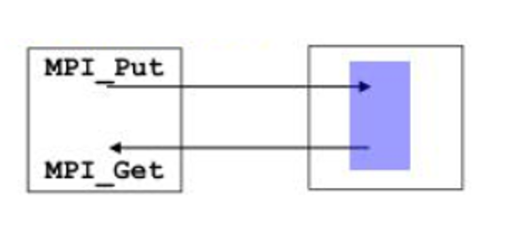
How About One-Sided Approach ?
This approach different from the master-worker because; without the need for functions such as send and receive, it can reach the specified areas and take it into its own memory.To initialize this area MPI_Window is used.Then other processes can reach and do put or get operation.
For our problem we want to have something like -Process 0 start and have 2 nodes.One of free process take one node from process 0 and compute.Each processes can share its nodes and so on.To make this we develop 2 version in one sided approach.
When process has more than 1 node;
Version 1: Inform the other free processes and one free process get this node
Version 2:It will look which process is free and put the node in it’s area
Comparison
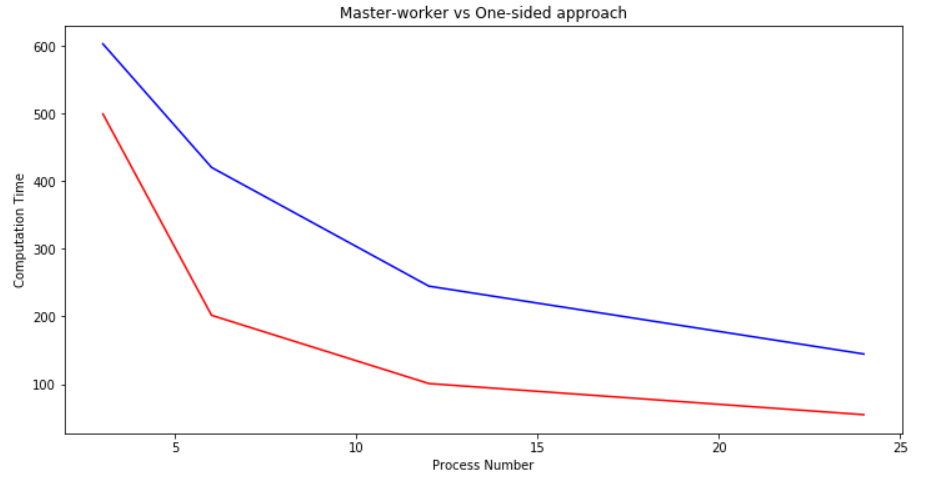
After implementing these approaches,we tested them with 130 different graphs.Below you can see the times of a graph that takes 955.37 seconds serially with 3,6,12,24 processes with master-worker and one-sided approaches.The results of the master-worker approach are better than the one-sided approach. The red line shows the result for the master-worker, while the blueline is the results of the one-sided approach.
The last week of PRACE’s High Performance Computing is just
about wrapping up, my colleague and I have just submitted our video
presentation and are now working on cleaning up the code and writing up the
final report.
Although all the models have been finalized and tested this week’s work is just as important as all the others. In these final days we are structuring the code and writing up documentation such that the work we have done isn’t lost over time, but can be taken over, integrated and used, as was intended, by our supervisors at Hartree Centre.
That sense of peace you get, when you are walking around late at night, the roads are deserted, you have published your video and you are finalizing your work – that sense you get when everything is coming together.
We are also working on the final report, where this has to
be written in popular scientific method. I have to say that I like this aspect
of the program, where both the presentation and report are to be written in
such a way that is accessible to a wider audience. Of course we have to put
some technical terms in there to explain all of the things we have executed in
our models, some of these aspects being potentially complex to the untrained
eye, but we do our best to explain these terms and why we chose the methods
that we did.
This has been the style that I have also been using in my previous posts, which you can find here. I can’t say if I would have found SoHPC’s program last year or not, without this initiative, or if I would have been immediately attracted or not, but what I can say now, is that I hope some other student stumbles upon these blogs, and our videos, and thinks: wow this is cool.
If you are reading this and debating whether or not to apply,
or if you have already been accepted and debating whether or not to go, I can
say it’s worth it. Sure it will be a lot of work, and over your summer break,
but the experience gained and knowledge learned is without question worth it.
Well, thanks for following along my journey, it is goodbye for now …
In the last blog, we discuss what a CNN is, what “flavor” of CNN we were using, and how we solved the issue of the cost function adapting the cosine similarity to work on our problem. Now it’s time to show how all of this work out in the training process and what outcome we archived.
The training process
To train the neural network we needed to structure the data in a way that is easy for the network to go through and understand. For that, we created a dataset with the normalized labels of the galaxies and the corresponding images. Once we have done that, we need to initialize the network with values for all the parameters. When the network has weights and biases we can feed data through it, see the results (at first all are gonna be random guesses), and compute our fancy cost function to see how far we are from the ground truth. When we have the error that we made we can update the network (change the weights, biases and kernels) with our optimizer. We chose the Stochastic gradient descent (SGD) as our backpropagation method.
Improving the dataset quality
As in any scientific process, we didn’t achieve perfect results at the first try. The first training runs were quite a mess. We started using the imagenet pre-trained weights. Then we realize that the images were too similar to each other and imagenet was always predicting the same output for all of them because the network was too stable to learn properly. Then, we changed to a randomly initialize network and the things went better (not by much). After that, we focus on one of the most important things in machine learning, the data. We restricted our dataset to just the galaxies more massive of 10^11 solar masses to have enough quality in our images, that made a significant change in our results.
Figure 1: Comparison between one galaxy of around 10^10 solar masses (left) and one of 10^12 solar masses (right). The different quality of the images is visible.
When 24 CPU’s is not enough
As we advanced in the project, the training runs take longer and longer each time on the CPU cluster. As this is a highly parallelizable task and is based on the perfect operations for a GPU, we moved all the training process to a GPU cluster with 4 Nvidia Volta 100. We went from 5h runs to 27 minutes… Not bad. But this not came without a cost. We needed to adapt our code to work in multiple GPU’s and to be extremely careful with the way we pass our data and update the weights to avoid possible conflicts.
The results
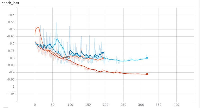
At this point, you may be thinking… Okay, but what did you get ??!! Okay, here comes the results. The metric we used is the adapted cosine similarity function where -1 is a perfect score and 0 is totally off and this is what we find:
Figure 2: light blue and red are validation and training of the resnet18 NN and the dark-blue and orange are validation and training of Alexnet NN.
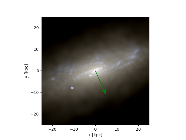
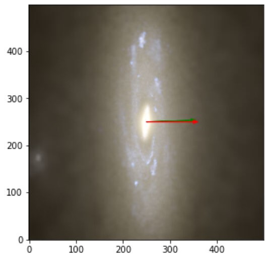
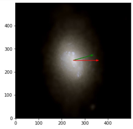
The images obtained with labels and predictions for the validation dataset are:
Figure 3: The green arrow represents the label and the red label the prediction. Notice that the first image is also a perfect score since we are looking for the axis of rotation and a 180º offset from the angular momentum vector is also perfectly align with the axis of rotation.
From there, and armed with all the things I learned in the SoHPC I will be looking for ways to improve this results and take it to another level… This was the end of the road but now I’m in the unexplored, the wild territory where real exploration is made. And thanks to the SoHPC I’m ready to face it.
If you are read my first blog post you should know I am an intern in SURFsara and this blog I will give you some basic information about HPC systems and what I do in Summer of HPC. Now, fasten the belds and be ready for my information overload about HPC!!!
Firstly, you should know about what is an HPC cluster? In short High Process Computing, but what is that mean? Please look at the photo below.
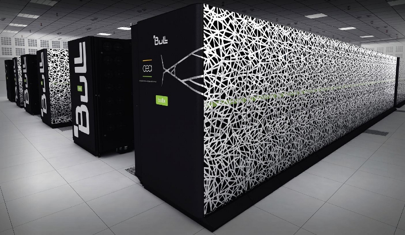
SURFsara Cartesius Supercomputer
This an HPC cluster or we prefer to say a supercomputer which is used in SURFsara. It was named Cartesius Supercomputer. Every weekday, I connect to the supercomputer from Turkey and make some tests, play with the system and gather some information on this supercomputer.
HPC clusters or supercomputers has a really good processing ability because they have too much powerful GPUs and CPUs which are connected parallel. This high process capacity using to make some scientific application for example an application ORCA which is about nano chemistry. Scientific use that for gather some information to their research.
If you want to make a test on a supercomputer, you should
know some parallelization tools. I use MPI and OpenMP in my internship. They
are used to make execute calculation on the parallel system. Otherwise, you can
just use a small processing ability of a supercomputer. For example, you have a big function which
needs too much calculation. You should use a program to split the function to
some small pieces for calculating these pieces in different nodes and after
executing the function, the program knows how to merge the all splitting
function pieces and give us an output. So the program can be MPI, OpenMP or you
can use both of them at the same time.
Now, you know what is HPC clusters, and what we use for parallelizing it. But the main problem is HPC systems are very heterogeneous environments. They have different parallelization approaches, different hardware solutions and there is a wide variety of scientific software offered to the system user. The heterogeneity is not a problem for just HPC maintainers, it is also a big problem for users. Because HPC maintainers should know that everything works fast, smoothly and reliable on their system.
For overcome this issue we use ReFrame framework.
I know that this explanation about ReFrame is not
understandable for beginners. So let’s see this scenario:
You have some input file and want to take an output, but you can not know how many nodes and how many tasks for each node you should use. Basically, you don’t know how to configure your test for using the system efficiently and take your outputs rapidly. Formerly, system user can make some configurations for tests, execute the configured tests separately and take this result and find the best performance… It is a time-consuming and very bad way to do it. Because the user will lose a lot of time while making these all configured tests. In SURFsara we use ReFrame framework about that. You can make some these tests in just one code file and execute it then it will give you all results in one file.
My first two assignment in SURFsara is about IOR and MDtest. Mdtest is a metadata benchmark tool, which is an MPI-based application. It can be used to evaluate the metadata performance of a file system.
What is metadata? If a book is a data then metadata is the book’s cover and contents. So basically metadata is a data which is summarize other data.
I can not execute mdtest while the system is working. If I try to execute it then file system might crash. This is because mdtest create new directories and enforce the file system for measure limit of the system.
And my second assignment is IOR((Interleaved or Random). It can be used for testing the performance of parallel file systems using various interfaces and access patterns.
In basic words, You can make some tests about IOR with using
and take outputs about the supercomputer write, read and remove performance.
Then, you can make a comparison and see when the performance is good. That will give you knowledge about your
system performance and you can detach any problem on your supercomputer.
I made the IOR tests on the Cartesian. Cartesian is a supercomputer which is placed in SURFsara. After took output of the IOR tests I am going to wrote some summarize according to the assignment.
Thank you for reading! See you again in my other articles.
Hello everyone and welcome to my last blog post of this Summer of HPC 2020. As I told you on my previous post, these last weeks of the summer I’ve been working on analyzing the performance of Alya.
Alya is part of the CompBioMed (European Centre of Excellence), and it is developed by the Barcelona Supercomputing Center (BSC). They were very interested in understanding how a new feature of their program behaves on Cartesius, so we collaborated with them to obtain meaningful metrics from the execution of Alya.
Logo of CompBioMed CoE
I especially enjoyed this part of my internship because in this case, I was helping not only HPC maintainers and users but also the developers to understand better how to improve their code.
Moreover, I was able to apply the methodology proposed by the POP Center of Excellence to analyse the performance of Alya. Particularly, we used the profiling tool MAQAO recommended by the POP CoE, and I helped to integrate its usage in the SURFsara workflow by creating a comprehensive guide on how to use it to follow the POP performance assessment methodology.
If you want to know more about what I and my mate Elman have been doing, take a look at the following video that we prepared!
Video presentation of project 2017
The end of SoHPC 2020
Everything comes to an end, and unfortunately, Summer of HPC 2020 is near to finish. It has been a very enriching experience which I have enjoyed even more than expected. During this summer, I have learnt a lot of things. Not only regarding HPC (which is what one would expect) but also concerning remote working with people from different countries, which I find even more important than HPC concepts. This new way of working was a challenge at first, but thanks to it, now I feel much more prepared to collaborate with teammates in this kind of environment.
Finally, I would like to thank PRACE and Summer of HPC organizers for giving us the opportunity of working on real HPC systems with top-level professionals and in an international environment. And of course, I want to thank my mentors of SURFsara for always being willing to help me with everything I needed and make the internship run smoothly.
This is all about my participation in the Summer of HPC 2020 program. I hope that you enjoyed reading about my progress in the world of HPC!
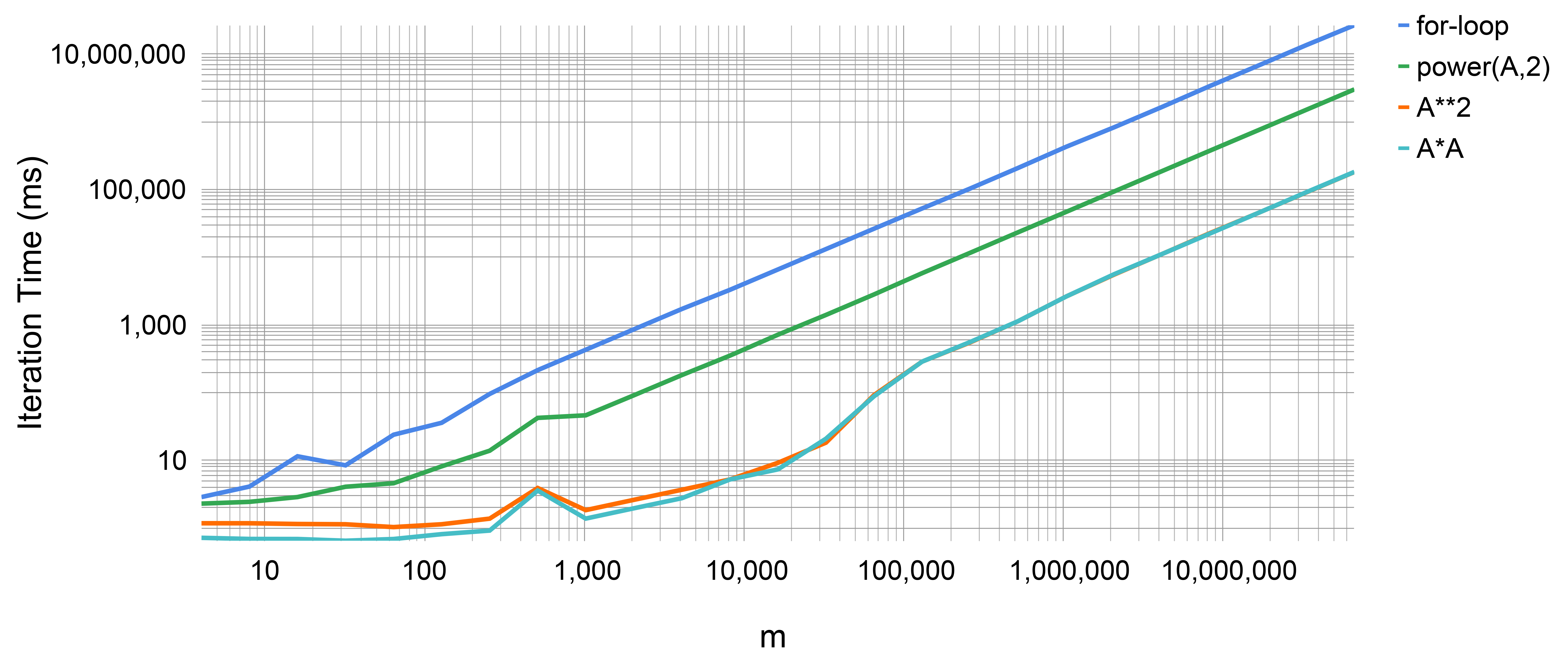
In this article, we will have a look at performance improvements on a very basic level. A program can be written in many different ways, (hopefully) always obtaining the same result. Still, the execution time may differ drastically. In higher languages like Python, one may not tell instantly, how a predefined function is implemented. We will discuss this issue on the basis of the square function.
As my college Antonis mentioned in his article To Py or not to Py?, we are optimising a python CFD program. For increasing the performance of a program, one does not always need to switch to parallel methods. One can start with simple things, like choosing the right implementation of a function. An important function of this project is the distance function. It is used to quantify the difference between the two matrices. It is used to stop the iterative process when the output is merely changing and therefore a minimum is reached.
The distance function uses the Euclidian metric. It calculates a scalar from the equally sized matrices and . This function provides a lot of parts to investigate. In this article, we will only look at the . You can investigate the rest of the function at home with the techniques provided.
To start we generate a random matrix of the size
import numpy
A = numpy.random.rand(m)
The square can be now computed using a for-loop
for i in range(m):
A[i]*A[i]
or the numpy.power-function
numpy.power(A,2)
or the python power function
A**2
or a multiplication
A*A
to just name a few. In IPython a code snippet can be easily timed with
%timeit [expression]
I wrote a script to time the previous functions for different sizes of , using the time-library. In the figure, the execution times of those implementations for different sizes of A are compared.
Iteration Time in ms over the matrix size m
Unsurprisingly the for-loop is rather slow. The simple multiplication may be up to one-hundred times faster. The numpy.power function is somewhere between. This may be more of a surprise. The numpy.power-function may be written especially for NumPy arrays. Of course, it provides more options and IS faster for larger exponents >70. For simple expressions like the square, an inline implementation should be chosen.
This post ends a series of reads related to ARM in the server space. If you are in the mood of some ARM-related tech, don’t forget to view the previous texts: ARMageddon: Really!!?? and ARM file I/O bechmarks and more.
OMPI under ARM
OMPI or Open Message Passing Interface is a library that guides the communication and the data flow when programming parallel computers, allowing the use of a cluster of computers to distribute the workload of a compatible program/algorithm. Right now, MPI (the standard) is the de facto programming model for the majority of high performance applications.
Everything was good until ARM wanted to join to the HPC party and requested its piece of the cake, and the following picture was the answer to that request:
The cake is a lie.
Yeah, confusing, right? Well, this describes perfectly how OMPI works under ARM.
First, OMPI expects some Intel-like-flavored numbering style such as:
Core 0 HW threads 0-3: [0-3]
Core 1 HW threads 0-3: [4-7]
Core 2 HW threads 0-3: [8-11] …
But, under the influence of ARM, the numbering style is as follows:
Socket 0 HW thread 0: [0..31]
Socket 0 HW thread 1: [32..63]
Socket 0 HW thread 2: [64..95]
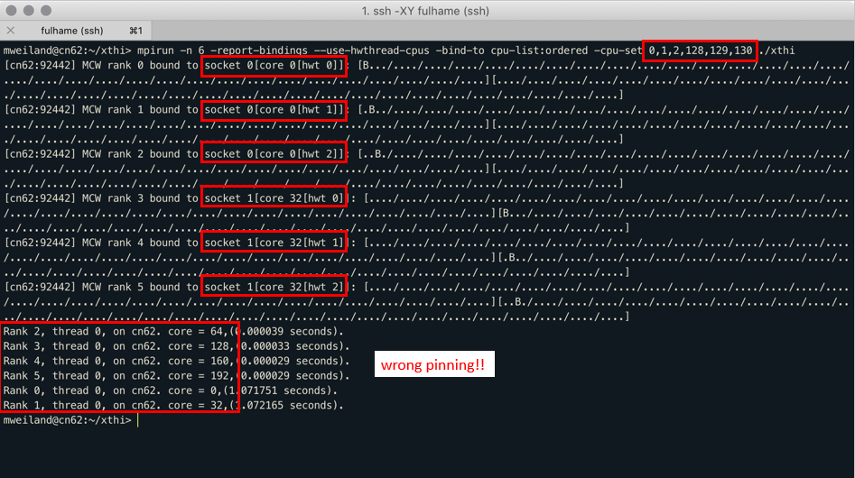
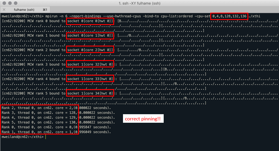
An example to demonstrate this problem are the following pictures, courtesy of Dr Michèle Weiland (EPCC) from the Catalyst meeting:
Due to this issue, the Fulhame cluster is running on SMT1 although it can run on SMT2 or SMT4, doubling or quadrupling its maximum theoretical performance®, or at least, the hardware thread count.
As you can wonder, yes, OMPI might need some tweaking to accept this nomenclature, but since I only had 2 weeks, studying the whole OMPI repository just to make this change happen wasn’t feasible.
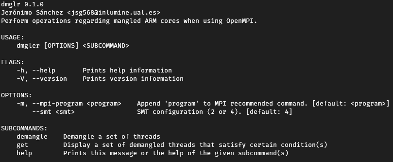
So, instead, I made a CLI tool, named dmglr or demangler, to sort of solve this issue.
dmglr usage.
It has various subcommands to demangle a set of given threads, or to get a set of them given some conditions.
The output of this CLI is a plain text line that contains a mpirun command with the correct or demangled input, just to execute on the cluster. This allows the researchers under the Fulhame facility to easily add the execution of the CLI on they slurm script and use the output to configure the node.
Closing thoughts about Summer of HPC
Before this global pandemic, I was in a summer internship at the IT department of a big company, sometimes feeling that I was bothering my peers and mentors, making them look after me or giving me made up jobs, etc. A sentiment of belonging.
When this opportunity came to me, I was still unsure about what to do during this summer (2020). When the pandemic arrived (luckily), the decision was not up to me anymore as the internship was cancelled, so the choice was crystal clear.
During this summer I have learnt about some of the problems that ARM is facing right now, just at the moment ARM has jumped from smart phones to PCs.
Aside of the technical specs of this programme, I really got along with my mentor and my colleague, although I still think that if the programme would have follow it initial plan, I could have made a friendship with my colleague and the rest of my peers of SummerHPC on EPCC.
I have nothing more to add than Summer of HPC is a really great experience both from a technical and a personal standpoint.
Today I come to tell you everything we’ve achieved during these two months with HPC! It is good news and I am going to tell it happily but at the same time very sad, the final week has come and we didn’t want it to come, all principles have an end and, of course, all endings are just the beginning of something bigger, and this is what has happened here.
New Family
At the beginning of summer, when it was announced that SoHPC2020 would go online because of COVID-19, it was bad news that would take the fun out of this great international internship. However, when you face a problem you simply get stronger. And that is why these two months have served to grow as people (#Stay at home), as students (#openACC, #HPC) and as researchers (#Julich, #Physics).
This has been the beginning of a new more virtual life that has also allowed me to meet many interesting people all over Europe, my classmate Anssi, my friend Jesús, my mentors Johann and Stefan,… with whom we share a passion, Computers! Thank you all!
GPU rules!
The positive side has been the amazing results we’ve obtained! To remember, in my previous posts (Cold start and Don’t stop me now!) you can inform in detail what is the work that I’ve developed during these months, which in short, was the export of an HMC code on graphene nanotubes from CPU to GPU using openACC library.
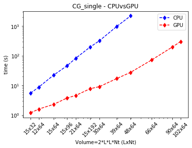
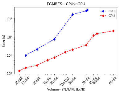
The hybrid method of Monte Carlo (HMC) with which we’ve been working, internally resolves dispersed linear systems calling two algorithms CG_single and FGMRES, developed by my colleagues at JSC. As a result of these systems presents the execution of a great number of instructions, we thought that it could be a highly parallelizable element.
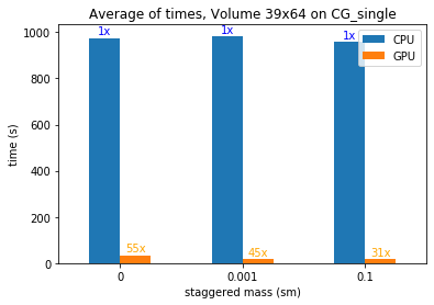
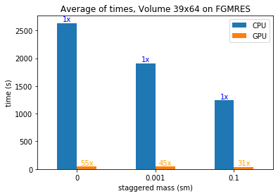
To show the improvement in performance and the importance of doing it well, we obtain in both solvers when we use GPU in their execution we’ve run two experiments for each solver. In the first one, we move the total size of the array, parameterized by the hexagonal lattice volume of the graphene, LxL with Nt timesteps. In these two plots, we can see the execution time required for the solvers CG_single and FGMRES, respectively.
In a second experiment, we leave the volume fixed and change the staggered mass (ms), another parameter that intervenes in the creation of the matrix A, in the next two figures we can evaluate the Speedup that we get.
Future works
For some future projects on GPU execution it would be very interesting to implement a version with CUDA and analyze what further improvements can be obtained.
Hello all! Here I am another day in a new blog entry. Today I will be giving some details about the simulations that we are doing in project 2019 and a brief description on our work.
If you do not know who I am or you want to read my introduction again, I leave a link here.
Why plasma kinetics?
Imagine you have 24 000 million euros (hopefully) and you want to invest them. After doing some research, you find out that you can build a nuclear fusion reactor called Tokamak which might be the best energy resource.
But you know that nuclear fusion is still in development and no one has achieved a stable and efficient reactor yet. The main issue that comes up with these reactors is the instability of the plasma (which is the energy resource of the core). And here is where plasma simulations take place. Obviously, you would not want to build a machine that may not work. Plasma simulations (in this case) give us the opportunity to track the plasma properties and be aware of its behavior, so the reactor’s structure can be adapted.
How are plasma simulations performed?
There are many kinds of physics models to describe plasma. In our case, and the most widely used model, is called Particle In Cell (PIC) code. These codes simulate each of the particles of the plasma. It updates each particle’s position, calculates the electric fields and many other features at each time step.
We want PIC codes to be the most accurate. To do so, they simulate up to 10 000 000 000 particles (10^10) and calculate electric and magnetic fields in thousands or more spatial points. So, by increasing the number of particles and grid points, our simulation will be more accurate.
HPC simulations
To add new plasma features and increase accuracy, more and more computational power is needed, but this is a limited resource. Here is where my work starts.
Most of the PIC codes run only on CPUs which limits the performance of the code because the computing time scales with the number of particles. To minimize these restrictions, the simulations can be carried out by GPUs.
Simulations in GPUs take the advantage of the large number of threads of this kind of device. Each thread performs one set of calculations independently from the others. For example, a standard (user distributed) CPU has between 6 to 16 threads while a GPU has 10000 or more threads. The key point to move a process to GPUs is to think of a way of make the computations independent. Also, you have to take into account data transfers between CPU and GPU.
GPU Simple PIC code work flow.
Adapting the PIC code to run in GPUs is not an easy task and this is what occupied my time during the last month of SoHPC.
Parallelizing the code
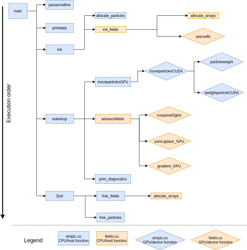
The main simulation depends on two processes which we moved to GPUs:
Particle mover: Updates each particle position and velocity and calculates the charge density at the grid points generated by the new positions. The CPU code is already independent as position and velocity of particles do not depend on the others. So, in a GPU we accomplish this calculation for each particle in an unique GPU thread which speeds up the code greatly.
Field solver: With the new charge density, calculates the electric potential is calculated bysolving a tridiagonal matrix and then the electric field is computed. For this process I encountered a new difficulty. I have to calculate the solution of a tridiagonal matrix system that comes from the discretization of the field equations. This is a dependent calculation, so it cannot be easily transferred to a GPU. To solve this problem, I used a basic algebra library from CUDA called cuSPARSE which contains GPU algorithms to sort out these problems. Also, the rest of the field calculations (computing the gradient of the potential to obtain the field values) are independent so, at this point, it was an easy task to implement.
Performance summary for particle mover calculations with a large number of particles.
Conclusions
We (my team partners Paddy, Shyam and me) have developed many versions of the PIC code to improve its performance. We have a CUDA (GPU) version, an OpenMP version and a hybrid CPU-GPU version integrated with StarPU. Now we are working in minor aspects of the code and bench marking for each version.
Stay tuned for the new posts, video and final reports to find out how this process has been made in more detail and which version has the best performance. I hope you enjoyed, see you!
Hi again, in the last post I explained to you the problem we are gonna address (predicting the orientation in images of galaxies), the motivation to address this issue, the technologies we are going to use, and the way we are generating our data. Now I’m gonna be a bit more technical and explain more in detail what model we choose, how it works, and how we are going to analyze the outputs to measure its performance.
Let’s begin with the basics
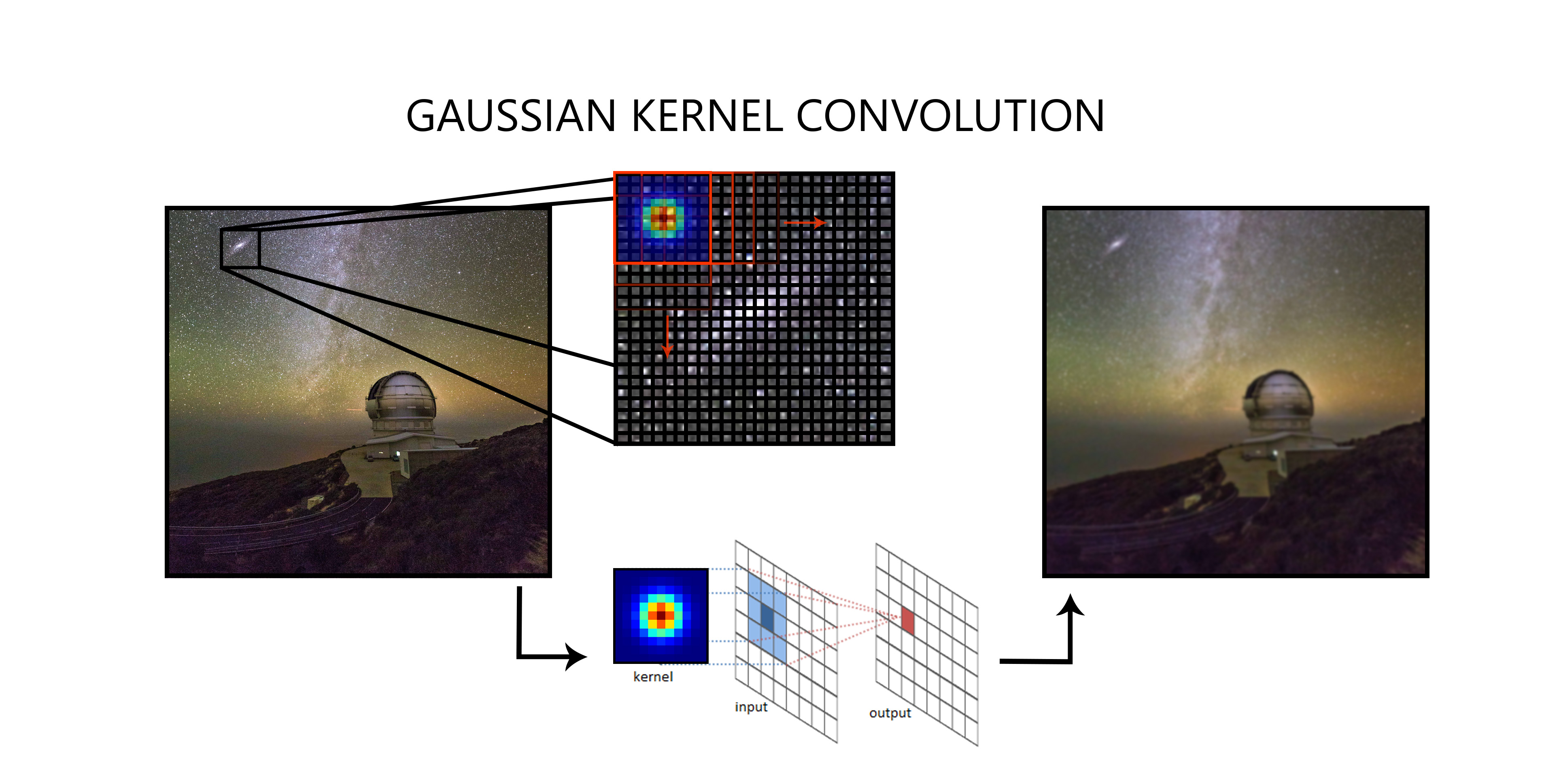
To do the actual predictions we are going to use a deep neural network, as we are treating with images the best option is to choose a convolutional neural network (or CNN for short). A CNN is based on applying a series of different convolutions on each layer. In case you are curious, convolutions are a kind of “filters” that are based on matrix multiplications as shown in figure 1. This convolutions then extract more complex features as we advance in the network to end up with a general knowledge of what features the orientation of the galaxy is based on.
Figure 1: Illustration of how convolutions work. The convolutions (the Gaussian is quite common) are also applied in image processing in common uses like photography.
A well-trained network is one that has figured out what the correct kernels should be to extract the information that we want. For example, in the first layer, the low-level features are extracted (like edges, corners… etc) then in the successive layers more high-level information is extracted (like combine edges and corners to have an understanding of general shapes) to finally have an understanding of what the orientation of a galaxy is. If we train the network we will end up with a bunch of convolutions that have been trained to extract the most useful features and will output as a result a 2D vector that represents the projected orientation of the galaxy into the image plane.
Time to do the heavy lifting
Now that we know the basics it’s time to choose the correct architecture for the network and with the right parameters. As we have time constraints and developing a new architecture from scratch it’s a really complicated task, we will use an already existing network. We first chose RESNET to do the job (we also considered ALEXNET). We chose these networks for being a state of the art networks treating with images but since our problem is not image classification (we don’t have categories) we need to adapt them a bit. For that purpose, we add a couple of extra layers at the end to adapt the networks to our needs of predicting continuous values.
Also, we need to develop routines to visualize the results, preprocess the data (shuffle it, batch it, and multiply it by applying flips and rotations).
Knowing how wrong you are is the first step to get it right
Okay now that we know what architecture to use, how we are gonna prepare our data, and how to visualize the results, seems that is almost done right? Well … of course is not that simple.
One key aspect of training a neural network it’s defining what is wrong and what is right and in a classification model, it’s a rather easy task since we have categories between which we need to choose. In a model like ours, in which we need to predict a real parameter (in fact 2 in this case), things get a bit trickier.
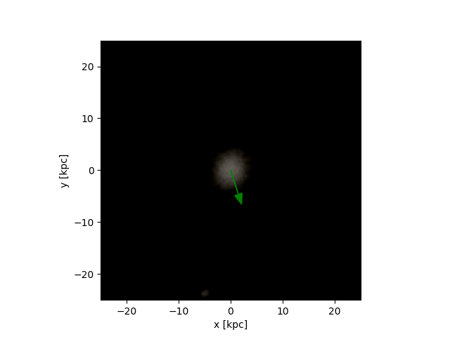
Figure 2: Galaxy showing the 2 possible solution vectors that we accept for the orientation of a galaxy.
We need to make a function that tells not if we are wrong or not, but by how much we are wrong. This gets even worse since we have multiple solutions for the orientation of a galaxy as the direction of the angular momentum vector can go in both directions of the orientation (axis of rotation) of the galaxy as shown in Figure 2. How we define how far is our model from reality then?
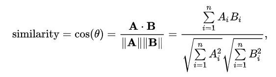
The approach we chose (as we are treating with vectors is to use the Cosine Similarity ( https://en.wikipedia.org/wiki/Cosine_similarity ) basically it’s a measure of the angular distance of the two vectors but taking into account that a +180º vector is a valid solution. It is computed with the dot product and the magnitude of the vectors A and B as:
From there we began a battle to obtain an accurate metric to train the network. Stay tuned to see what the results of this amazing journey are … See you on the finish line.
DNA sequence alignment algorithms use heuristics methods in order to cope with the high volume of data that is passed to them. These approaches, usually run on super computing clusters, take days to finish due to the amount of data, and usually with an approximate solution. This permissiveness with the solution makes these algorithms possible to work with quantum processors. (See more in detail information here.)
In our project, we mainly focused on the string encoding and comparison. For the alignment, we decided to work with a naïve approach, but of course, further improvements could be done using a better algorithm. Regarding the original project idea, I want to remark that we ended working with Qiskit from IBM instead of Forest from Rigetti, so that would be a small change regarding the quantum computing software platform.
Of course, before start with the encoding and comparison, it was necessary to understand some quantum concepts and how quantum computers work. If you are interested in that I really recommend reading Benedict’s post, where he explains some basic concepts that we have to understand before getting hands-on.
Encoding
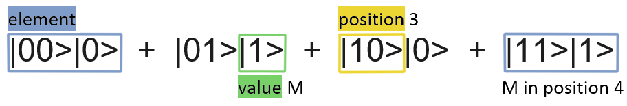
Getting back to what we have been doing this past week the first challenge we face was trying to encode the strings using Quantum Registers. For this task, we divided the information between the position of the element in the string and information about the element itself.
Both pieces of information need to be translated into binary. For positions 0 for the first one, 1 for the second, 10 for the third, … and so on. For the values of the elements, we need to know how many different values are in the string. If there are just two values, one would be represented by 0 and the other by one, if there are four: 0, 1, 10, 11 would be the binary versions of each of the different values.
So, let’s put an example: we want to encode the string ‘-M-M’. We have 4 positions to represent 2 different values. If we use 0 to encode for – and 1 for M:
Summary of encoding ‘-M-M’ string
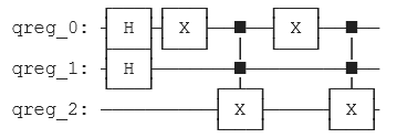
Quantum circuit with ‘-M-M’ string encoded
We applied the corresponding operations to encode the strings in a Quantum Circuit. To save memory, we used some properties of quantum computing, such as superposition.
Comparison
Regarding the string comparison, we base that on a simple idea. We initialized all circuits at 0 for every Quantum Register. Once we have applied the operations to encode the string, if we applied the same operations but in reverse order, the initial state of the circuit will be obtained, with all registers at 0.
Therefore, when we want to compare 2 strings, we are going to add the operations of the second string in reverse. And then, we will check for the Quantum Registers, if all are at 0, that would mean that the 2 strings are identical. The more different the strings are, the more 1 will be found in the quantum circuit. For example, if we compare ‘—-’ to ‘MMMM’ we will obtain that all registers are at 1.
What is left to do?
More or
less we resolved these two challenges for DNA sequences, and in a way that can
be more or less general for strings with different information. Now, we are
left to do the final implementation and measure performance.
Hello everyone, I hope you are all well and with your loved ones during the pandemic period. After SoHPC’s rapid introduction to my life, I set out to advance the project. There were concepts I know a little, but I was motivated to deal with artificial intelligence.
The Beginning of My Journey
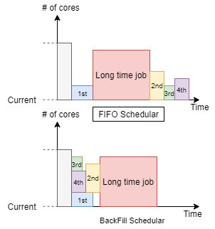
Figure 1: Comparison of FIFO and Back-filling scheduling algorithm
As I mentioned in my previous post, me and my teammates Francescawere developing an algorithm to determine the time limits of the jobs people submitted to supercomputers. In this way, jobs won’t be thrown to the end of the queue due to back-filling optimization. If I briefly explain the back-filling optimization:
When the workload manager (SLURM) receives long-term jobs, it controls the nodes to execute them. SLURM manages time usage efficiently by sending short-term jobs to idle nodes. A simple visualization of the back-filling optimizations is made in Figure 1. However, because users enter the time limit much more than the elapsed time, SLURM considers these jobs as long term jobs and assigns the job to the end of the queue.
My Travel Pack
Figure 2: Normalized Elapsed time and time limit ratio of submitted jobs
We have provided a database of the job batches of the supercomputer of Hartree center to develop the regression algorithm. The data provided are nearly 2-year job distribution data of 5 users. As seen in Figure 2, some of these users are people who determine the time limits of their jobs reasonable, and some of them give their limit times higher than the elapsed time. With this feature of data, we had to make an appropriate prediction for both types of users.
Where am I on The Road?
When the project started, our motivation was to complete the project with the least extra resources. In this way, users will be able to use the project without using much extra resources. For this reason, I prepared two regression model from scratch and a regression model created with sklearn.
What Awaits Me on the Continuation of Journal?
We have achieved considerable efficiency in time limits with our predictions, but our current goal is absolutely no underestimation in the time limit predictions.
Apart from the paperwork, we can learn to apply a regression similar to our short-term jobs in our own daily life. In this way, we can create extra time for our hobbies. For example, I like to play my guitar when I wait for things to happen on the computer. So, what are the back-filling optimizations you do in your daily life?
Hello everybody! I am really excited writing this blog post – I have some cool stuff I want to share with you. If you missed last time’s post, I described what the project is about and mentioned one optimization for the serial Python code. Today’s topic – as the featured image reveals – is how code parallelization can be applied to accelerate a program.
Why to have parallel programs?
Imagine that you have to mop the floor in your house. Would it be faster if you did it all alone or if you got help from your family so that every family member mopped one room? If your answer is “Well, it depends…”, you are overthinking it. It is obviously faster to have more people (processes) mopping one room each (running the program with one part of the input).
Ways of parallelization
In this project, I have used MPI (Message Passing Interface) programming to parallelize the CFD (Computational Fluid Dynamics) simulation program I explained in my last blog post and achieve a speed up on CPUs. Additionally, I developed a GPU version of the program using CUDA programming. Now, let’s see how both of these programming models boost the performance of the CFD application.
Using MPI
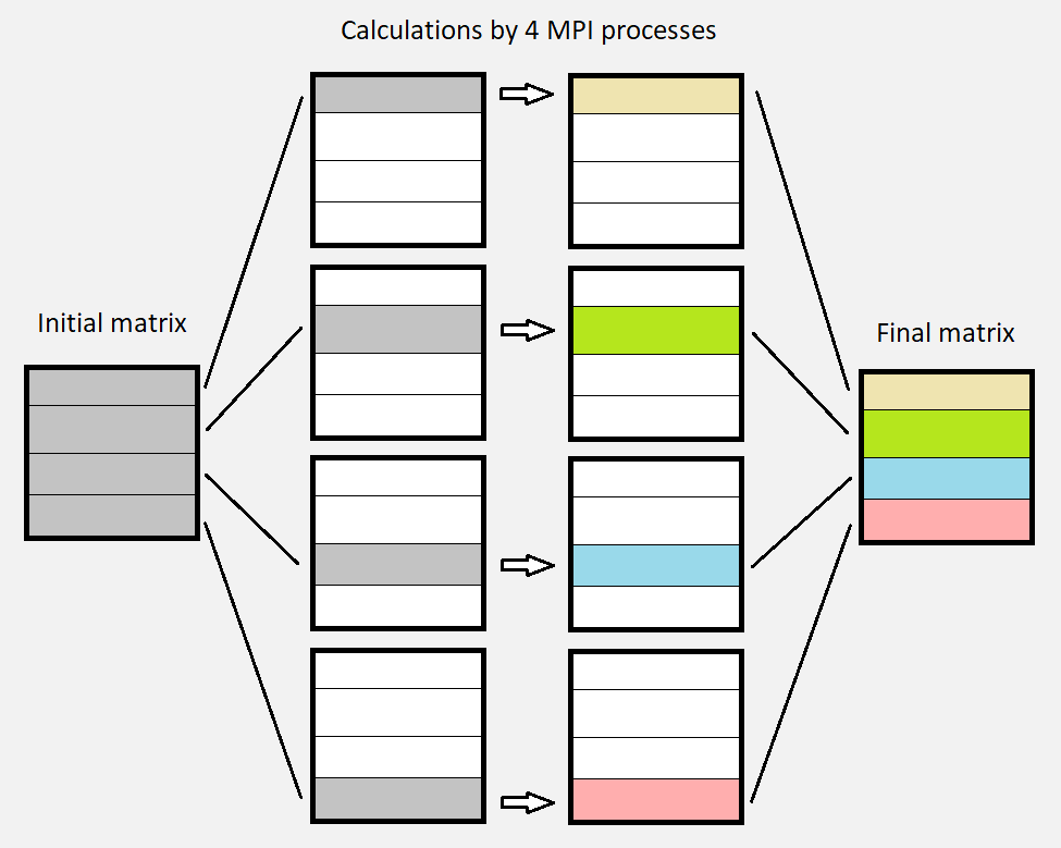
One really effective way to speed up the program is by using MPI processes. Previously, there was only one process doing the whole work, i.e. the calculations on the entire matrix. Now, there are multiple processes each responsible for one strip of the matrix. These processes are working in parallel and produce one strip of the final image (matrix). In the end, these strips are combined to form the whole final matrix.
Example where the calculations are made by 4 parallel MPI processes, each one affecting one horizontal strip of the matrix.
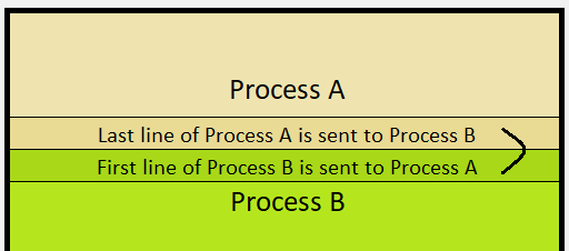
There is a communication between processes A and B to ensure that both have access to the data they need. When process A calculates its last line, it needs the line below that, which is the first line of process B.
There is one detail for this technique to work properly. Because every point of the matrix uses the four neighbouring points to calculate its own value, there is an issue for the boundary points between two strips. This can be solved by sending data (messages) from one process to another.
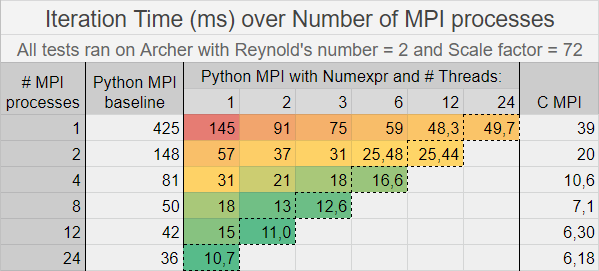
MPI programming model can be applied on both C and Python. So, I added MPI parallelization to the optimized Python code with numexpr module and compared its performance with the baseline Python MPI code and also the C MPI code. The conclusion of this performance analysis is that the numexpr MPI Python version is significantly faster than the baseline one and close to the C MPI. Moreover, it seems that the performance gain by increasing the number of threads is not as big as by increasing the number of MPI processes.
The red to green gradation reveals the cases with the best performance for the optimized MPI Python code. The marked diagonal contains cases in which all 24 cores inside a node in Archer are used. (Cores used = MPI processes * Threads per MPI process)
Using CUDA
In recent years, there is a trend to use GPUs not only for gaming but also for general purpose, especially for programs that make few decisions but do many calculations. That’s a logical thought to make if you consider that instead of running tens of parallel MPI processes on the CPU, the GPU offers the ability to run thousands of threads in parallel. In our case, the optimal is to assign every point of the matrix to a separate GPU thread. The whole matrix is stored in the GPU’s memory, so any thread has direct access to any point of the matrix without exchanging any messages like MPI.
Python Numba CUDA
For the Python code, I have used Numba CUDA to implement and launch kernels (functions) on the GPU. Algorithmically, the procedure for each iteration is described by the following pseudocode:
for iterations number do
    (step 1) calculate new matrix using the current matrix
    (step 2) calculate error between current and new matrices
    if convergence == true then exit ‘for’ loop
    (step 3) copy new matrix to current matrix
end do
These steps have to be sequential because of the dependencies of the matrices. That means that all GPU threads executing one step in parallel have to finish before they continue to the next step. Currently, Numba CUDA doesn’t support thread synchronization, except if the threads are in the same block of threads. But we need to synchronize every GPU thread and having just one block is not considered optimal. The only way to achieve synchronization between all threads is by launching a different kernel for each of the above steps. But this is not optimal either, because there is an overhead for each kernel launch. The ideal would be to launch just one single kernel to execute the whole ‘for’ loop instead of launching 3 kernels per iteration. That’s the reason why at this point I shifted from Python to C.
C CUDA
C CUDA offers the opportunity to synchronize all GPU threads, by considering them to be in the same cooperative group. In this way, the program can launch one single kernel and be fully optimized.
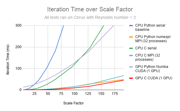
Iteration time over Scale Factor (size of the problem) for serial, MPI parallel and GPU program versions written in either C or Python.
Conclusion and Question
I am excited to be part of this project and I am happy I made quite a lot of progress in the last few weeks. However, it is not always easy with programming. I’ve spent about 5 days debugging the C CUDA code. So, my question for you this time is:
What is the max time you have spent to debug a program? Please, feel free to share in the comments your most intense debugging experience. As always, thank you for reading my post. I am looking forward to seeing your comments.
It’s been just over a month of working on my project and I’ve just about got my head around the concepts of GPU programming using CUDA. In this post, I will try to explain some concepts of my work using everyone’s favorite analogy – FOOD!!! Let’s get into it then.
CPU vs GPU: What’s the difference?
Imagine that you are the head chef in a 5-star Italian restaurant, which serves the best Lasagna on the planet. Of course, the Lasagna is going to be the most ordered dish in your restaurant. And due to the soaring popularity of your restaurant, you begin to receive a crazy amount of orders (say around 1000 Lasagnas) every hour. You could sweat it out and make each Lasagna, one by one, baking each of them to perfection. However, at the end of one week, you’re absolutely stressed out and are not able to handle this volume of orders everyday. Now, this is where your manager comes and helps you out, telling you that you can recruit 100 junior chefs to help you to get those orders out faster. However, the catch is that, the junior chefs are not ‘that’ well trained to make decisions on their own. You can however give them instructions and they will follow them to a T (sometimes even faster than yourself!).
This is the difference between a CPU and GPU. You are similar to a CPU. You can operate independently using your logic and get work done, but only one order at a time. The group of 100 junior chefs you’ve recruited, that’s how a GPU works. There’s not much independent logic and everyone in the group does the same work that they’ve been instructed to do. But given the right instruction and facilities, you can get a whole lot more work done using the group. Now, let’s see how the actual work can be distributed among our new recruits.
Making Lasagna vs Moving Plasma Particles
A VERY ROUGH(!) ANALOGY OF THE PARTICLE IN CELL (PIC) CODE I’M WORKING WITH
The entire Lasagna recipe can be roughly broken down into three important stages as can be seen above. Let’s try to distribute the work in the three stages.
Pre-Processing
Let’s assume that this stage involve cutting, sauteeing the vegetables, meat and preparing the sauce. So before you can give instructions to your army of chefs, you need to assemble all the chefs together to explain exactly what needs to be done. Also, you need to distribute the ingredients equally among each of the 100 chefs. Once the junior chefs have the ingredients and the instructions, they can each go to their individual workstations and get to work!!!
Is this the best way to go ahead? We need to see if the time taken for you to work alone is lesser or more than the time taken to assemble the chefs, distribute the ingredients and then for the chefs to finish. We can safely assume that distributing the cooking among 100 chefs would easily take less time than one person working on 100 dishes despite the extra time required for assembling the chefs and then distributing the ingredients. So yes, you can breath easy now. But wait, your manager tells you that the number of orders are doubling every day!!!! Now, the amount of ingredients you need to distribute becomes humungous and this alone takes a lot more time than before.
One of the reasons you have been made head chef is that you can come up with solutions to such problems, and EUREKA!!! You have come up with a very simple solution to it all!!! Why not just give each of the chefs the list of ingredients and ask them to get the ingredients on their own. Then, you remove the distribution step completely and they can start cooking immediately. YOU GENIUS!!!!!!
How does this compare with the particle in cell (PIC) code I’m working on? When we need to call the GPU to do some work, we need to first call the special code (instructions) we’ve written for the GPU and then transfer all the data for each ‘worker’ in the GPU to work with (distribute ingredients) from the CPU. These codes run with a huge amount of particles (>1000000000 particles!!!!) and you can imagine that transferring this data would take a lot of time relatively. To solve this problem, we simply create these particles in the GPU itself (similar to how each junior chef gets their own ingredients).
Processing
Now the lasagna needs to be baked. However, the problem is that the restaurant is still using the one oven which you have in your workstation. So each of the half-finished lasagnas need to be brought to you first. But luckily the oven you have is absolutely high-end and efficient and you are still able to manage the large amount of orders!!! PHEW!!! But afraid that the number of orders might increase further, you approach the manager asking if we can afford individual ovens for each of the junior chefs’ workstations. She says that we could do it, but the ovens wouldn’t be as good as the current one. You’re now stuck in a dilemma! Is it worth investing in 100 individual slower ovens or do we continue with the extremely fast oven we still use? You also understand that it depends on the number of orders you receive. If that keeps increasing, it may be a good idea to invest in this. If the orders stay the same or decrease, you could still continue working as before without further investment.
Again, let’s compare this with our PIC code. The code for this step currently has a very serial (can be done only in a certain sequence) but extremely efficient and fast algorithm to solve for the fields. However, you can try to change the algorithm completely in such a way that each ‘worker’ in the GPU can work in parallel. It might not be the most efficient algorithm, but it could be faster than the initial version if the number of particles we have is bigger. Contrarily, you’ll need to give extra instructions to the GPU which also takes some more time.
Post-Processing
Now that the lasagna is ready, you need to make it a 5-star dish. And since you’re the head chef, only you can add the finishing touches and check if everything is right with each lasagna. Hence, if each of your junior chefs has his/her own dish, you’ll need all of them to assemble and go through each of them one by one. Unfortunately, this can only be done by you and hence, this step cannot be avoided.
Some of the cool visualisations from the OOPD1 PIC code!!!!
Similarly, in a PIC code, all the calculated results in the GPU need to be transferred to the CPU so that the required data can be extracted and presented to the user in a cool, visual manner. Unfortunately, this can be done only on the CPU for now.
Final Word
Throughout the last month, me and my teammates Victor and Paddy have tried out all these different methods of work distribution between the CPU and GPU and checked which ones give us the best results. ( If you have more novel ideas for similar work distribution, please mention them in the comments below!!! ) We’ve managed to get some exciting results which we will present at the end of this month. Stay tuned for this!!!! All this talk about food has got me craving for some authentic Italian food. I’m off to satisfy my hunger along with a cold beer to beat the summer. Till then , Ciao Adios!!!!
Hello again, this time from my hometown of Kavadarci, and welcome to my second blog post about my remote, summer internship at the CINECA research center in Bologna. As I have already described in my previous post, this summer I am working on a project to detect anomalies in the work of the Marconi100 cluster at CINECA.
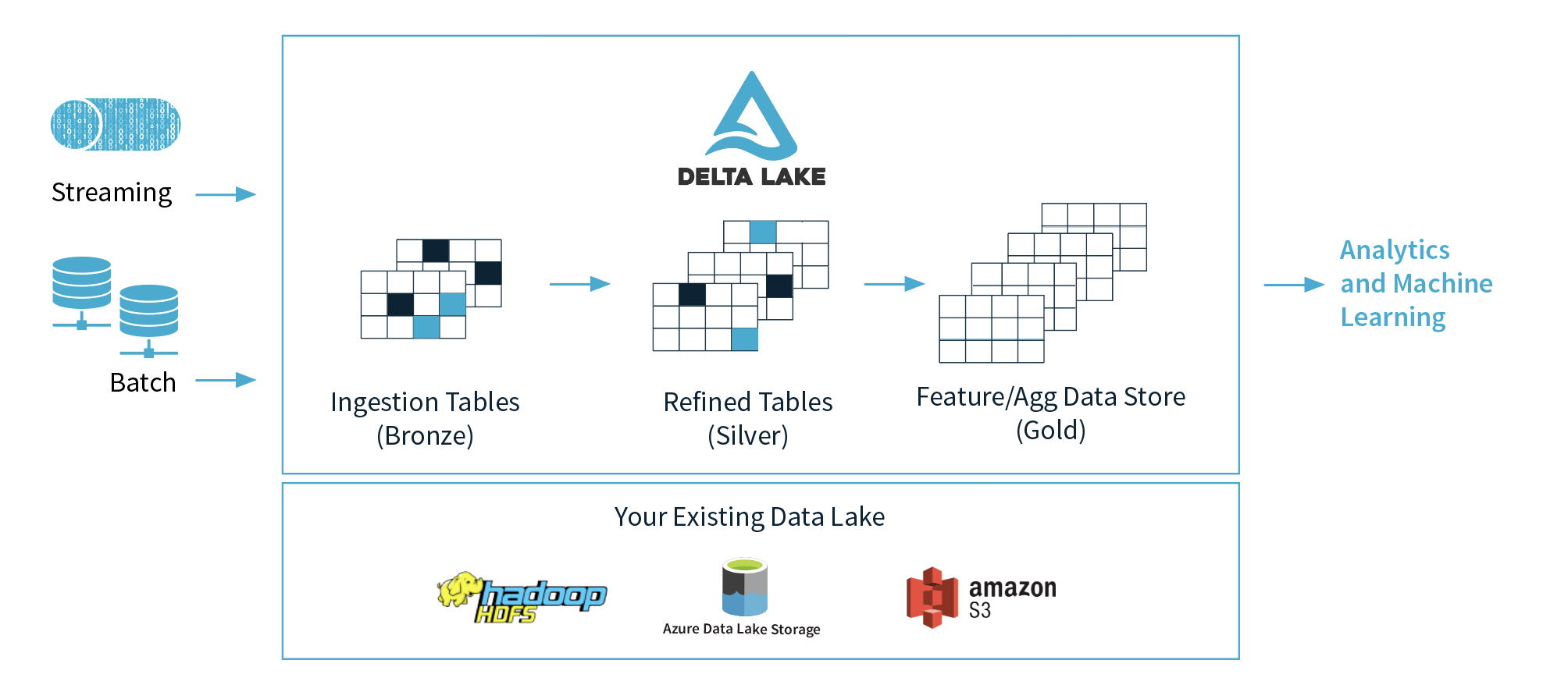
My job in this project is to gather the data set on the Marconi100 cluster that contains information about nearly every environmental factor that impacts it’s working performance and store in Delta Lake format.
Delta Lake marketecture. Taken from http://delta.io/.
Delta Lake is an open-source storage layer within the Apache Spark engine that offers ACID (atomic, consistent, isolated, durable) transactions to its big data workloads. A major feature of Delta Lake is to enforce the schema of the data set during writing; something that has been missing so far from Spark. Another really important feature is that Delta Lake works seamlessly with Apache Parquet; that is – it stores the data in column-oriented format which is substantially faster than the more-common, traditional row-oriented format.
Consider for example a question that might arise from this data: Plot the temperature of node X for May through August 2020 and check if there are any anomalies (unusually high or low values) in it? In the traditional row-oriented format, the processing engine would have to read a batch of rows, and for each row it should scan up to it’s N-th column (where the temperature is stored) and this could take a while, considering that there might have been many columns in between that can be large in memory and force the engine to read more disk blocks. Now with the column-oriented format, each temperature value is stored right next to each other and reading the column data can be very fast (fewer disk reads). Also, we would need less storage for the data, because there are techniques for compressing it (each column contains homogeneous data). In big data scenarios, column-oriented storage is the way to go.
As the project is coming to an end, I am hoping that there will be enough time to use this data to train a machine learning model to automatically detect anomalies. Stay tuned to read about it in my next blog post.
Hello again, and welcome back to my PRACE SoHPC blog! In case you missed my introductory blog post, you can find it here. Last time around, I mentioned that my project this summer at the CINECA HPC facility in Bologna deals with the visualisation of supernova explosions in a magnetised inhomogeneous ambient environment. Over the last few weeks, I spent a considerable amount of time familiarising myself with the Galileo cluster at CINECA, learning how to edit and run models on the supercomputer. The supernova explosion models were run using The PLUTO Code, a freely-distributed software for simulating astrophysical fluid dynamics.
Starting with the basics
Once I was comfortable implementing sample models on GALILEO, I began running the simulation of an exploding supernova (SN) and the subsequent supernova remnant (SNR). I firstly considered the case of a spherically symmetric supernova blast wave expanding in a uniform circumstellar medium (CSM). The CSM contains the mass-loss from the progenitor star that was stripped away by the stellar wind in the years leading up to the explosion.
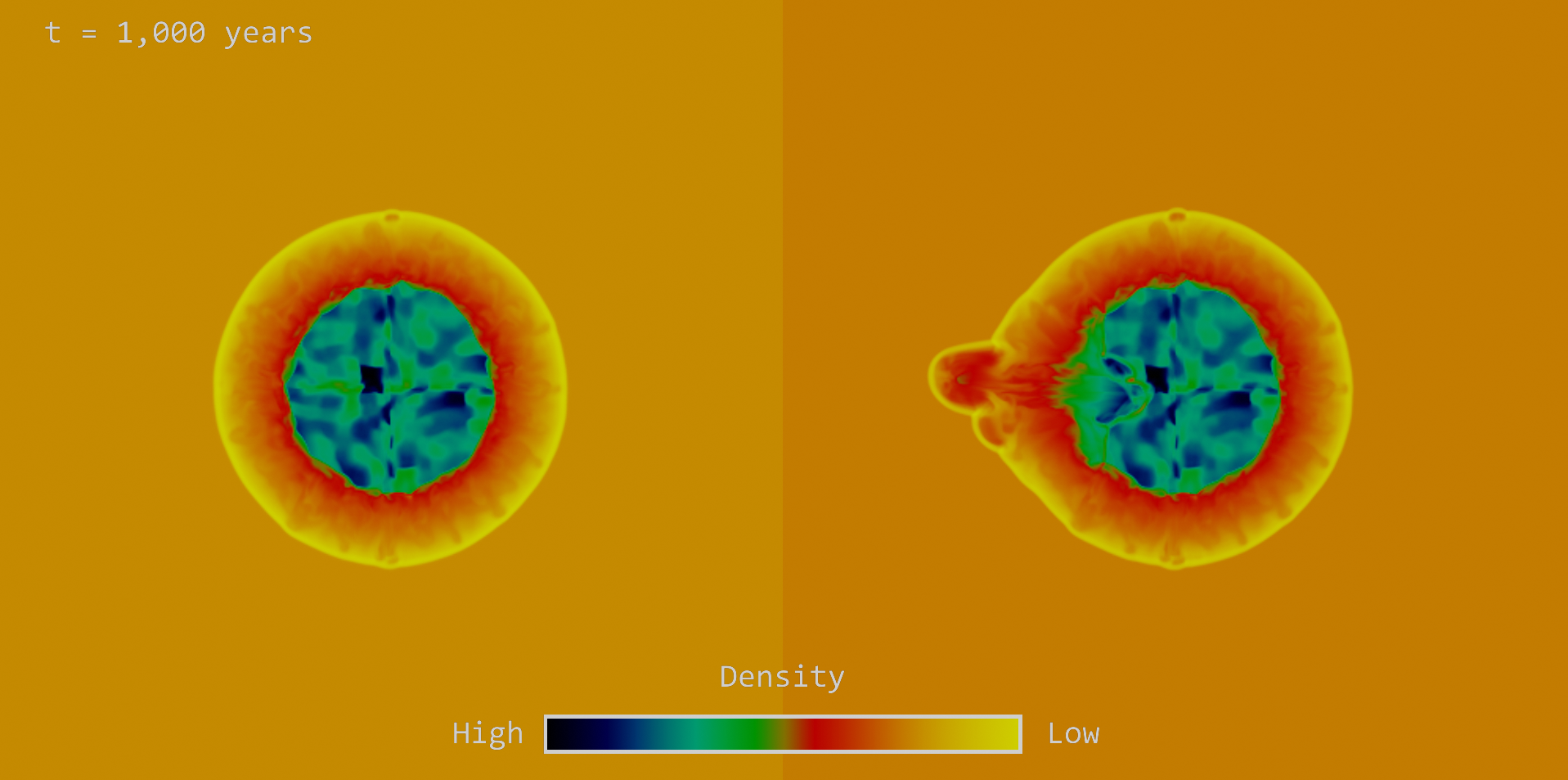
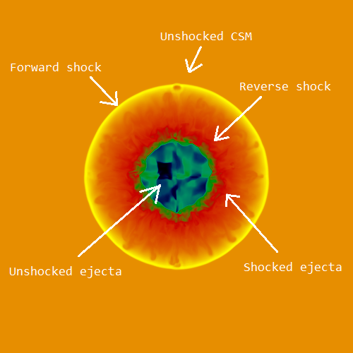
When the expanding SN ejecta interacts with the CSM, some of the material will continue to propagate outward in what is known as the forward shock. Conversely, some of the material will travel backwards into the freely expanding ejecta after colliding with the CSM. This is known as the reverse shock. The diagram below shows a 2-D slice of the density profile of the remnant at a time of 1,000 years since the supernova explosion, and each of the regions are easily distinguishable.
Schematic diagram of the density profile of a spherically symmetric SNR in a uniform ambient environment at a time of 1,000 years after SN explosion.
One of the input parameters that was defined in the model was the density of each of the regions. In the image above, the region with the highest density is the unshocked ejecta (blue) at the centre of the remnant. If we then move outwards, the density drops off as we go to green and then to red. The orange/yellow colour of the unshocked CSM represents low densities (as expected, as this region is much larger and has less mass than the remnant).
For a better sense of the evolution of the blast wave, scroll down and check out the short video below!
Making things more life-like
When I was happy with the shape and evolution of the symmetric blast wave, I began to introduce asymmetries into my model to make it more realistic in comparison to SNR’s that we have observed (such as Cassiopeia A). As a first step, I added a clump of material to one side of the initial remnant. I set the density of this clump to be 10 times greater than the rest of the SN ejecta, and the velocity of the clump was set to 5 times the velocity of the ejecta. The image below shows that the effect of this clump is to cause a protrusion of the outer remnant, distorting the remnant compared to the spherical case that we saw earlier.
Comparison between the density profile of the symmetric (right) and asymmetric (left) blast waves at a time of 1,000 years after SN explosion.
The video below shows the comparison between the two models as they evolve over time.
Evolution of the density profile of the symmetric (left) and asymmetric (right) blast wave explosions. The simulation runs for 1900 years, and the movie clearly shows the expansion of the blast wave, the forward shock and also the reverse shock on interaction with the CSM.
What’s next?
For the remainder of the summer, I will continue to introduce more asymmetries in my models to better resemble real-life SNR’s. This can be achieved by adding more clumps, all of different sizes, velocities, and densities. Another possibility is to add asymmetries in the ambient environment, and this area is being investigated by my colleague, Cathal Maguire. Check out his latest blog here, where he attempts to include a torus (doughnut-shaped) feature within the CSM.
I will also spend more time analysing my models using the 3-D visualisation software Paraview. Finally, I plan to upload my models to SKETCHFAB, a platform for publicly sharing 3-D models. Exciting times lie ahead!
Hello again and welcome back! Though it’s only been just over a month since my last post, a lot has changed. Here, I’ll try to explain some of the stuff I’ve learnt, what a general computational fluid dynamics (CFD) simulation is and how one is carried out.
The learning process of completing a CFD simulation is made easier by working with examples further down the simulation line and working your way back up. This is how I’ve learnt to complete the simulations. That being said, I’m worried that writing about the process in that order may make things a tad confusing for the reader (let alone for me writing this). Instead, I’ll explain my experience in the order you’d perform a CFD simulation. Just remember, if you’re considering learning how to do these too, do it in reverse!
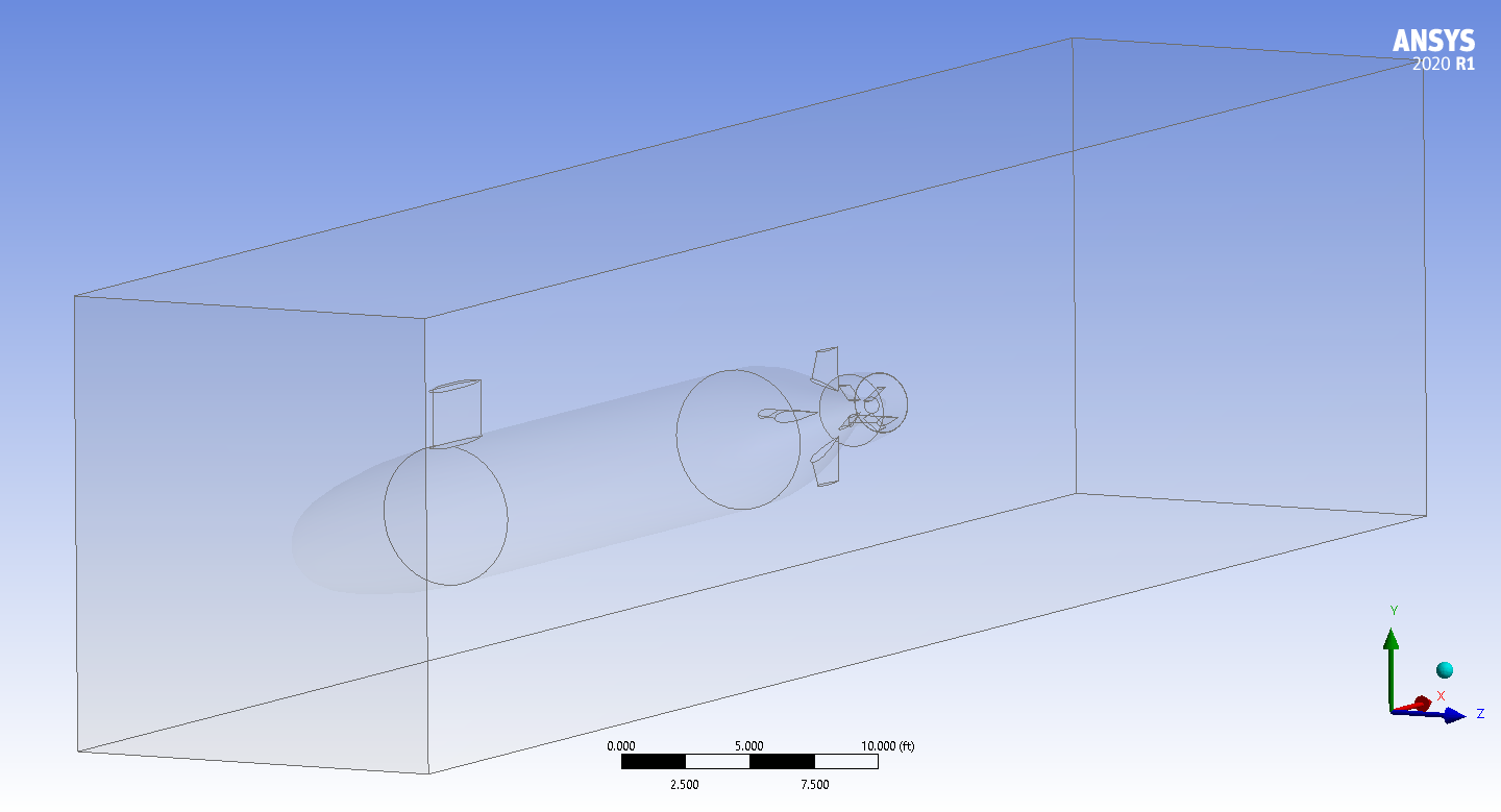
To begin a CFD simulation, you must first define the geometry of your problem – which quite literally means defining the shapes involved. Fortunately, this can be easy when working with simple shapes, like a cube or sphere. Unfortunately for me, submarines can be quite difficult to draw freehand and I was never very good at art. I was thankful to find out that the submarine we are modelling, the DARPA Suboff, has its geometry specifications online which, with a little Python and a lot of luck, can be used to produce the complete geometry in a format we can use.
However, to perform any simulations on this, we have to specify boundary conditions (BCs). These BCs include where the fluid is coming from (inlet), where it exits (outlet), and where fluid can go (fluid domain) in the simulation (we’ll come back to these later). With just the submarine in the geometry, we cannot specify where the inlet, outlet, or fluid domain are as the only object that exists is the submarine.
The way CFD fixes this, is by using cavities. This involves creating a large volume in the geometry that encases the submarine (such as a cuboid or cylinder), and then making a submarine-shaped hole inside it. This means we can say the inlet is the front face, the outlet is the back face, and the fluid domain is the volume of the shape that remains after removing the submarine. At this point, it’s important to remember, the fluid cannot enter the cavity. Instead, the fluid domain is just the surrounding volume.
Apologies that this one looks so dull, but this is the backbone of the entire simulation. I promise they look cooler further down the post!
After this, we create a mesh from the geometry. Meshing is a form of approximation that allows for the CFD calculation to take place. This involves splitting the geometry into a set of finite chunks so we don’t have to consider a continuous space. The smaller the chunks, the finer the mesh. So far, the default mesh generated by ANSYS has worked perfectly fine (thankfully), but this may change more precise simulations are required.
An example of meshing a sphere. Each level increases the fineness of the mesh.
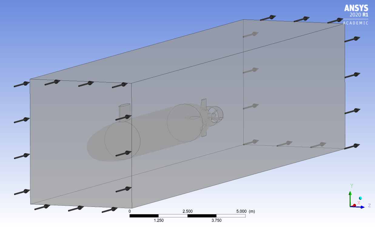
The next step is to set up the problem. This involves setting up all the BCs. However, there are many more than the ones I mentioned earlier. These BCs include how the fluid should interact with each face of the geometry, the static pressure of the fluid as it leaves the outlet, and the initial velocity of the fluid. And we still haven’t considered the array of different solvers & methods that can be selected. It goes without saying that that there were a lot of important decisions to be made here, which meant I had a lot more to learn! This involved a bit of reading about CFD and a fair amount of trial and error. As I am writing this, the conditions for my final simulations are still undecided, but I know I’m on the right path.
Program display once BCs have been set. You can see here where the inlet and outlet are defined, along with the walls of the simulation.
Once that’s all done, we can begin performing the simulation. Since we have access to an HPC cluster, we can complete such a task much faster with parallelisation – which is quite the upgrade from performing the simulation in serial on your local PC. Those working at the HPC cluster in Luxembourg have done a great job at making the IRIS cluster accessible considering the circumstances. Since most of the heavy lifting has been done in the setup process, at this point the only thing to do is sit back and wait for the cluster to crunch the numbers.
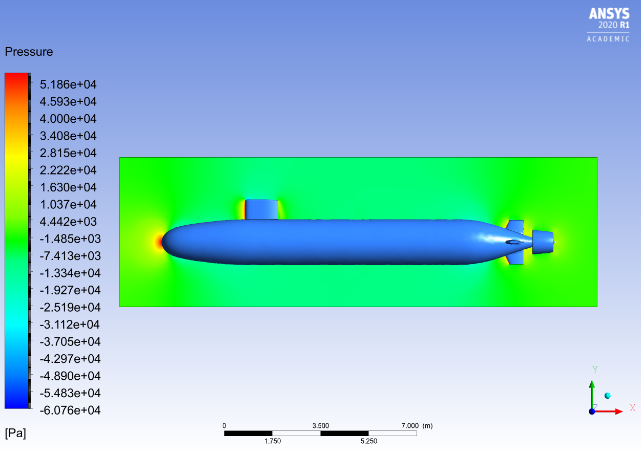
A contour map of the pressure in the water surrounding the submarine down its middle.
Finally, we arrive at the most exciting part of the process. At this point we see if the conditions we set prior have correctly shown the physical properties we were after – or if we’re heading back to the drawing board. Once the files have transferred from the HPC cluster to your local PC (during which time you could learn an instrument, or count the grains of sand at your local beach) the post-processing begins!
While I initially learnt how to post-process in Paraview, I decided to switch to ANSYS since it’s built into the ANSYS workbench. Within these programs, you are able to select the physical quantities calculated (such as fluid velocity, pressure, temperature etc.) and visualise them on the geometry itself. This allows for a very useful sanity check, as we can see if the simulation has given us physical behaviour, plus we can look at some very cool looking pictures and videos! However, we do still have to work out if what we have simulated is the correct physical behaviour. This means outputting the numerical values of our simulation and comparing these to the values to those calculated in the DARPA Suboff model experiment.
How the turbulence surrounding the submarine evolves with time from 0 to 5 seconds. You can see how most of the turbulence is due to the turbine at the back!
As it stands, I have two weeks remaining to complete the project and can already smell the sweet scent of correct BCs in the air. Hopefully all goes to plan… and I’ll provide an update on the final results in a couple of weeks!
Thanks for reading! Any questions, please let me know in the comments below.
The above Prometheus architecture diagram gives a very good overview of what our Time Series Monitoring system looks like. The architecture is divided in three main components.
The Prometheus Target is a http endpoint where a script is being executed which creates metrics from information produced by a job or service running and makes these metrics available over the above http endpoint.
The Prometheus Server makes a pull request (scrapes) from the Prometheus Target http endpoint for these metrics created by the executing script. The metrics scraped are stored as Prometheus’ own flexible query language called PromQL.
Data Visualization of these metrics is created by executing a pull request of metrics stored as PromQL from the Prometheus Server. The resulting PromQL can be parsed and refined by the end user and displayed on graphs.
Job Queue Exporter
The Job Queue Exporter acts as the Prometheus Target. Information we are interested in is job queues of HPC schedulers. Two main schedulers exist for HPC systems: Slurm & TORQUE. Because Slurm is the most well known and used scheduler, the rest of the post will focus on the Slurm squeue command which returns information on job queues for the Slurm scheduler.
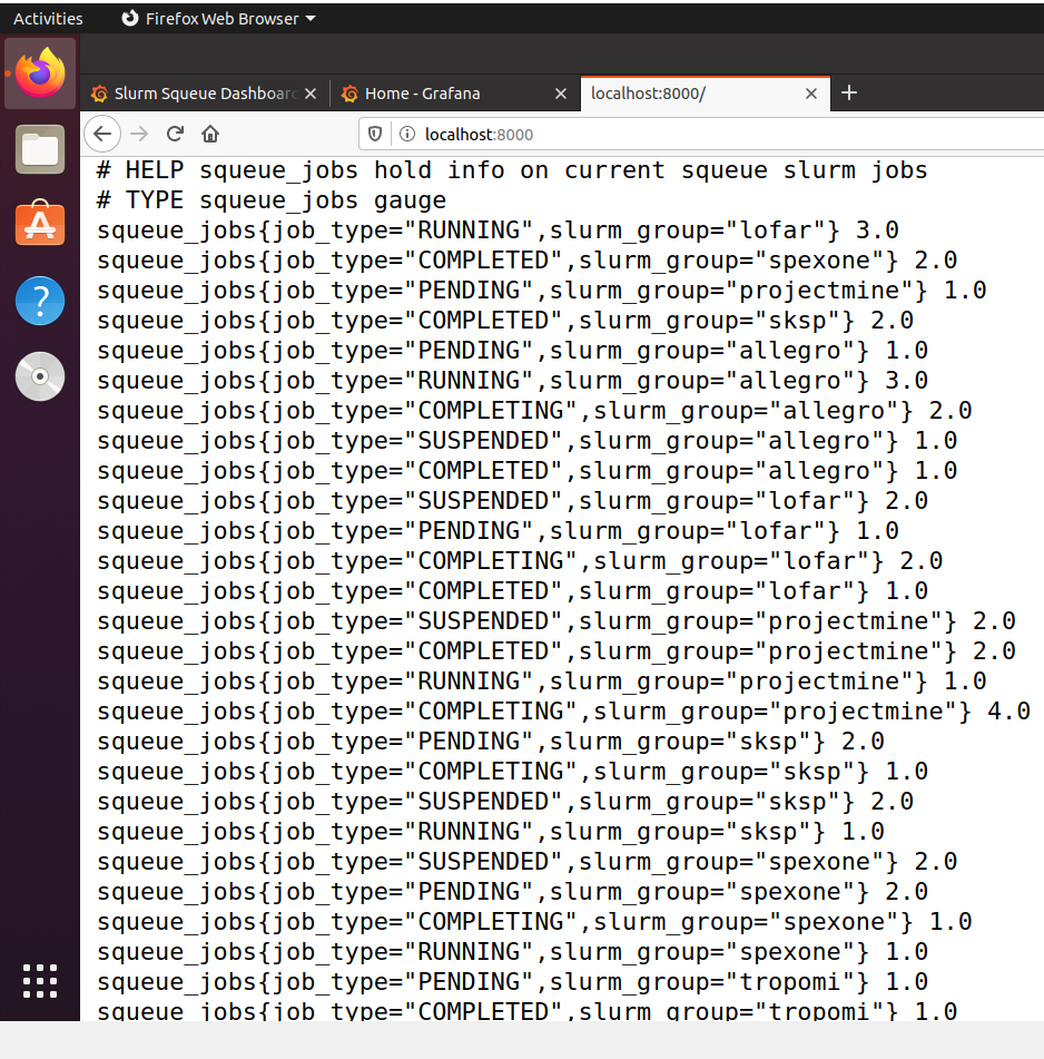
The exporter is a Python3 script running which executes the squeue command, retrieves information on job queues running, converts the information into a Prometheus Gauge Metric and makes the metric available over http://localhost:3000.
The exporter has been created as a Python pip package and can be installed through pip3 install job-queue-exporter or the source code is found here. Unit testing of the exporter used pytest and tox testing tools.
Sample Prometheus Gauge Metrics from Slurm Squeue Information.
Prometheus Server
Fortunately, the Prometheus Server takes care of all the scraping of the exporter http endpoint, processing of metrics and storing of information in PromQL which leaves very little to worry about for the developer.
The number one file in configuring Prometheus is prometheus.yml which specifies all the Prometheus Targets, their associated http endpoint where metrics are exposed and scraping time interval. The prometheus.yml file configured for our system can be found here and the result can be found at http://localhost:9090/ where Prometheus is running by default.
Other information can be configured in the prometheus.yml associated with Prometheus Rules and the built-in Prometheus AlertManager system . One rule configured for our system is when a Prometheus Target experiences downtime, the system maintainer can automatically be notified over email or Slack and can take the correct measures to revive the failed node.
Prometheus creates pull requests to the Exporter, Grafana and its own metric endpoints.
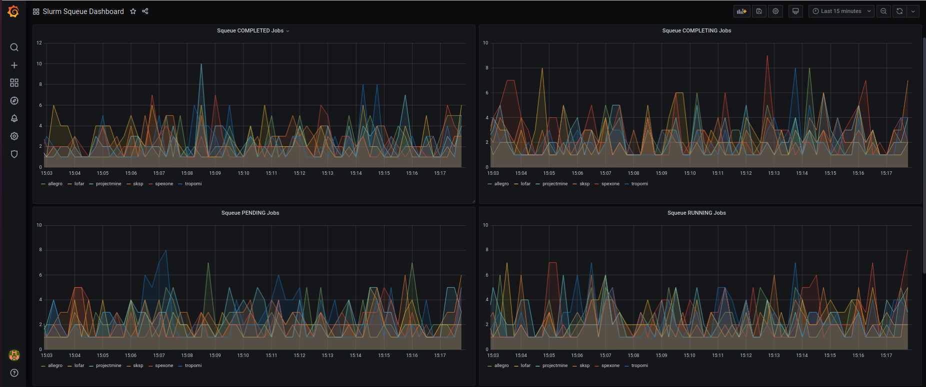
Grafana Data Visualisation
The Prometheus Web UI can be used to visualize Prometheus PromQL queries. However, Grafana is a more elegant and stylish data visualization software that is compatible with Prometheus. Two tasks need to be completed before getting nice dynamic graphs of job queue information.
Configure the Grafana Data Source to pull from the above Prometheus instance running at http://localhost:19090/prometheus/
Configure the dashboard which is stored as JSON data.
Our graphs are created through Prometheus PromQL queries in the following format: squeue_jobs{job_type=<job_type.name>} which creates graphs for individual job queue types. The graphs can be further inspected by clicking on an individual {{slurm_group}} in the graph legend.
The guys & gals at SURFsara can now view job information in visually appealing graphs. Next steps involve collecting data from the graphs to determine if any time series trends or statistical properties occur when jobs are run on SURFsara HPC machines.
Resulting Grafana Graphs of Job Queue Information.
Full System Deployment
Ansible is the open-source software provisioning, configuration management, and application-deployment tool enabling infrastructure as code that fully automates deployment of the above system with the click of a button.
In addition to running the above tasks, the Ansible playbook configures Prometheus and Grafana to run behind a reverse proxy. Often, machines have a limitation, due to firewall policies or other security reasons, only opening to the external world ports such as 80. If you take a closer look at the above Prometheus Targets running on the server, it is evident that Prometheus is actually running over port 19090 instead of 9090 and Grafana over port 80 instead of 3000.
If interested, full deployment details of the system can be found over at the following repository.
In machine learning we often talk about accuracy as a metric for how good our model is. Yet a high accuracy isn’t always a good way to measure model performance, nor does it always correlate to an accurate model. In fact, an accuracy rate that is too high, is something to be skeptical about. In machine learning this is something that comes up time after time, you build a model, you get a great accuracy score, you jump with joy, you test it further, you realize that something was wrong all along… you fix it and get a far more reasonable answer…
Side note for the inexperienced reader, if any model or any
person tells you that their model predicts the target variable with a 100%
accuracy… don’t believe them! How big is their sample size? Are they training
and testing their model on the same dataset such that the algorithm simply learns
the answer? Have they tested their algorithm on all data we have available for
the topic throughout human history? In short, what’s the catch?
In this post I will be talking about how the accuracy metric wasn’t useful in the models I have been building to predict SLURM job run times. In fact, the accuracy metric could even be counterproductive in some scenarios. If you remember from the previous post, estimating predictions of actual job run times could greatly improve the efficiency of Hartree’s cluster scheduling algorithm.
The first model I built was a regression model, given information from the user, like how many CPU’s and nodes they request from the cluster, and what they expect the run time to be, the model tries to predict what the actual run time of each job will be, whilst minimizing the error in prediction. Now in this case, the classic accuracy score isn’t applicable, for regression prediction, things like MSE, mean squared error, are used to estimate the goodness of fit achieved from the model. In the figure below on the left hand side, we can see the red line is the line of best fit for the scattered points. This line minimizes the distance between estimated and actual points. In our case, the line of best fit becomes a bit more complicated. The algorithm my colleague and I are building has the obligation to predict run times such that no run time is underpredicted. That is because in Hartree, similar to many clusters, if the actual run time of a job goes above the provided time limit by the user, the job is killed. So the first and foremost necessity our model has, is that it cannot predict run times lower than the actual time, otherwise the job would then be killed. On the right hand side of the figure we can see how this would look like, the line of best fit is shifted upwards such that no points fall above it.
A typical line of best fist on the left hand side, the right hand side modifies the line of best fit such that the line lies above all points.
Now this figure represents a simplistic example, but it is a good way to visualize the problem. In real world problems though the data is much more messy, there are outliers, in both directions that would skew the line of best fit. For our dataset we have an additional complication though, which is presented by the fact that even users sometimes make errors. Users will occasionally submit jobs with runtime predictions that are too low, causing the scheduler to kill their job. These jobs are highly unpredictable and will almost never be accurately estimated by the algorithm. Due to this limitation, we decided construct another model, this time to tackle a classification problem. The idea behind this is that if we were able to classify jobs into two categories, predictable and unpredictable, then we could simply put aside the unpredictable jobs, and run our regression model on the rest, without risking under-predictions and having jobs killed off.
As such we ran our regression model and defined accuracy as
whether the run time was predicted correctly above the actual elapsed time (but
below the user’s time limit), or incorrectly below it. Having these two
classifications we constructed and tested other models like Random Forest
Classifier and Naïve Bayes Classifier, to predict the “predictability” of a
job. With the accuracy we defined before we had roughly 92% of jobs classified
as predictable, and 8% as unpredicatble.
In the first run of a classifier algorithm the code spat out 92% accuracy!!…. Well, that was easy? In fact, too easy. Since algorithms are built to train in such a way that they achieve the highest possible accuracy score, Naïve Bayes simply predicted every job as predictable….oh, so we got 92% accuracy, but in reality that was useless? Yes, the whole point was to distinguish the jobs that are unpredictable, and even with such an “accurate” algorithm, we were nowhere nearer to achieving that task.
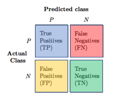
This is one of those scenarios where accuracy scores are misleading. In this case we want to achieve 100% accuracy in predicting “unpredictable” jobs…but remember, what’s the catch? To do this we have to sacrifice accuracy in predicting those jobs which actually are predictable, and misclassify them into the other category. The below image helps to clarify. In our case, think of jobs being predictable as the positive class, while jobs that are not predictable are part of the negative class. Traditional accuracy only looks at the diagonal values of jobs correctly classified as positive or negatives. Other metrics, like recall and precision, take into account the other diagonal of false predictions. In our case we want precision to be 100%, this means that we do not tolerate any false positives (such that negative cases are all correctly labeled). To achieve this though we will generate many false negative cases.
A confusion matrix displays the true and false categorization of classes. In this case the classes are only two, positive and negative.
This is it for now folks, we have cornered the best tactic to achieve no under-predictions and now what remains is to optimize the models best we can and test such models on the cluster. We are slightly passed the mid-program mark but I can see the deadlines for the final week approaching. Working on this project has been an amazing experience so far and I have been learning so much thanks to SoHPC, but it’s not time to relax yet .…


^2}") . It calculates a scalar
. It calculates a scalar  from the equally sized matrices
  and
and  . This function provides a lot of parts to investigate. In this article, we will only look at the
 ^2") . You can investigate the rest of the function at home with the techniques provided.
. You can investigate the rest of the function at home with the techniques provided. of the size
 can be now computed using a for-loop