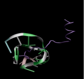
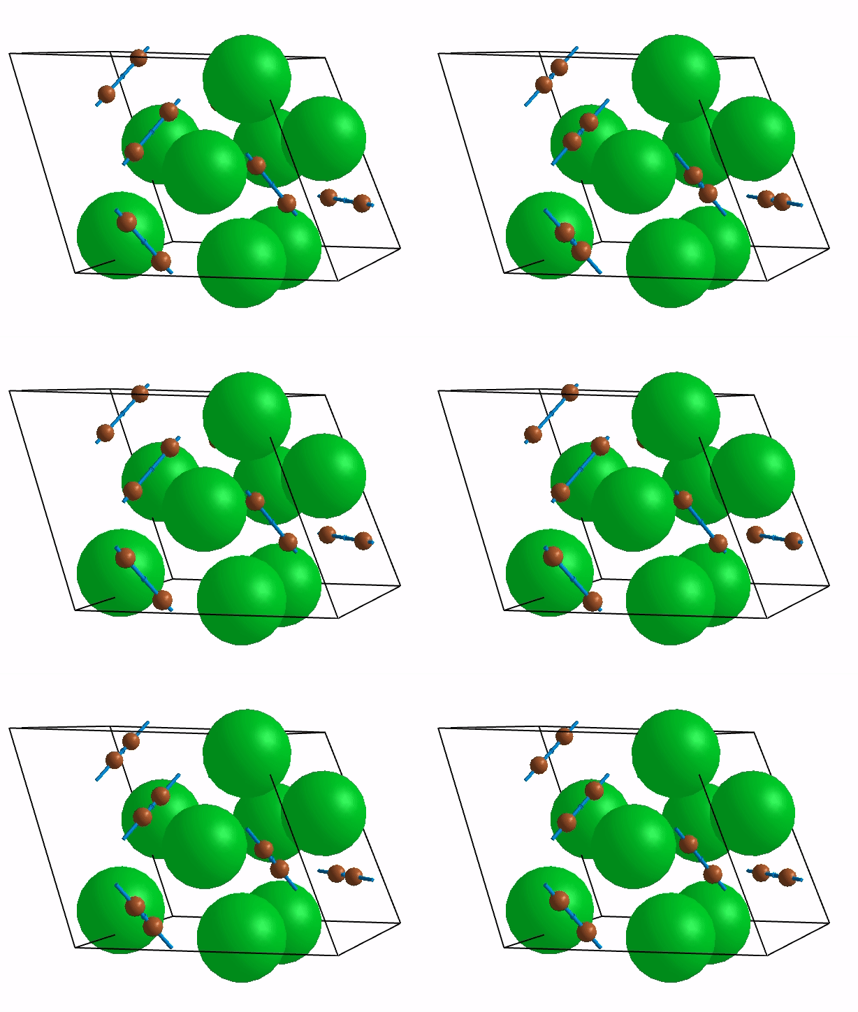
Figure 1: TAT-M178 MD image taken from MD simulation

As I mentioned before, this project aims to develop a drug against viral ds-DNA, which is associated with Herpes Simplex Virus, Cytomegalovirus, Adenovirus type 5, SV40 Polyoma virus and Vaccinia virus.If viral DNA is blocked, it cannot replicate inside the cell. Targeting virus DNA is more accurate, but it can also bring disadvantages.

In our study
We use the well-known TAT from HIV ; I24 is a 9-mer amino acid sequence that can be fused to TAT. Here, random mutations were obtained by making single-point mutations in the sequence of TAT-I24. New mutant peptide sequences obtained by single point mutations were subjected to MD simulations (250 ns).

After the MD simulations, the MM-GBSA and MM-PBSA binding free energies were calculated. Molecules with high MM-PBSA and MM-GBSA scores can be used as drug candidates in the next step.

While doing MD simulations

Molecular Dynamics Simulation (MD) tests the interactions of molecules in the system for a certain period of time by making calculations.In the MD simulation performed here, DNA and peptides were tested in a explicit water solvent and simulated for 250 ns. Therefore, the interactions of atoms and molecules during this time were tested. We benefited from AMBER/20 and GPU performance while doing MD simulation. In this way, we performed more MD simulations in a shorter time. As a result of MD simulations, 250 frames were obtained. We viewed them in a video. We observed that structural changes occurred between molecules with good MM-PBSA and MM-GBSA (ΔG) scores. There were particularly strong interactions between ds-DNA and mutant ligands.

MM-GBSA and MM-PBSA Calculations

After MD simulations, MM-GBSA and MM-PBSA binding free energies are calculated. Here; MM-PBSA uses the Poisson-Boltzmann equation to calculate the electrostatic contribution to free energy; MM-GBSA uses the Generalized Born approach. However, we cannot compare the speed between MM-GBSA and MM-PBSA. This may vary depending on the parameters we use. The lower the energy obtained in these Computational experiments, the stronger the interaction between the molecules. Therefore, TAT-M178 gave the best results with -103 kcal/mol (MM-GBSA) and -76.6 kcal/mol (MM-PBSA).

Figure 2: Frame 0 (TAT-M178)
Figure3: Frame 100 (TAT-M178)

We had 120 variants of TAT-I24. We performed MD simulation for each of this variants. As a result, TAT-M178 gave the best score.

In Figure 2 (Frame:0) , that is, they are not fully interacting at the MD starting point, but in Figure 3(Frame:100) , There is already strong interaction between TAT-M178.

Unfortunately this moment had to come, and to be honest I barely felt the flow of the time during these 2 months here at Luxembourg, was a really ephemeral summer. But let’s go straight to the good news and present my collaboration for XDEM developer team.

I am very thankful to present my contribution which will be part of XDEM Continuous Integration which is important to
ensure and maintain the performance of the software with new versions of the code, we automate the process of per-
formance analysis and regression detection. In this way developers could check if the changes affect the performance of the simulation, and highlight the part of the computation which is impacted.

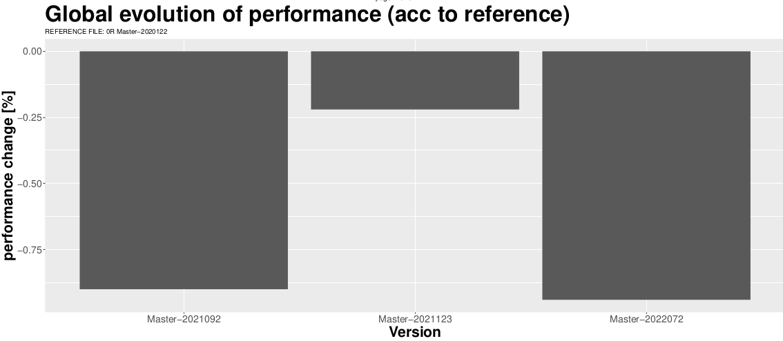
Barplot shows how performance changes across versions, normally for software development it is okay to sacrifice a little bit of performance if the implementation gets modular and easy to understand.

The data acquired to test the performance report is from a blast furnace charging simulation, this involves intricate physical phenomena that must be modeled (and validated) carefully and require the use of High-Performance Computing (HPC) platforms which in this case is Aion cluster at ULux. For those curious there is a video with a graphical representation of the simulation.

This report points to answer the following questions:

  • Strong Scalability: If I have two processors instead of one, will I get done the job in half the time?
  • Weak Scalability: Will two processors finish twice the job as in done with only one processor?
  • Complexity characterization: How the computation time increases according to the size of the problem?
  • Performance regression: Are there crucial changes between different version of XDEM?
  • Decomposition comparison: How the execution performance differs with different workload distribution methods?
  • Workload balance: Does every node do the same amount of work?
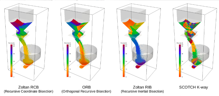
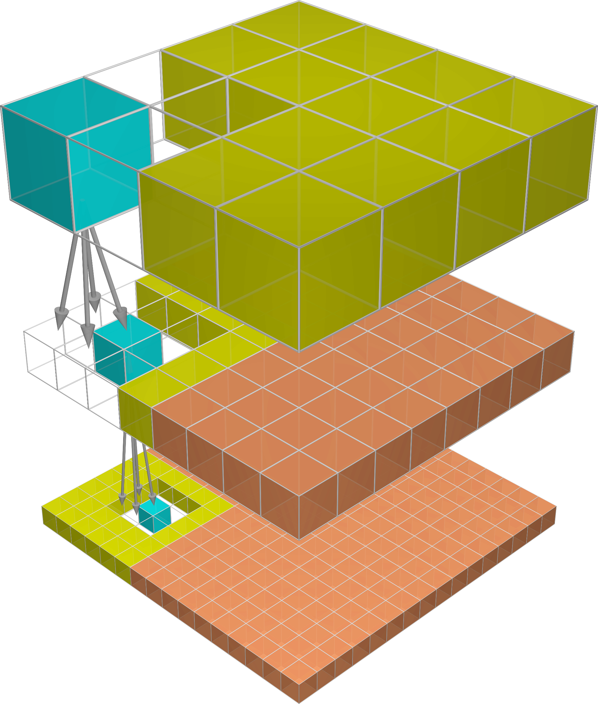
A graphical representation of different decomposition methods. Different color, different node.
Decomposition matters 😉

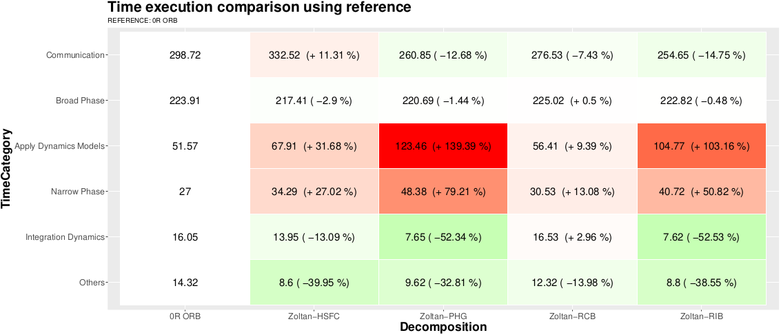
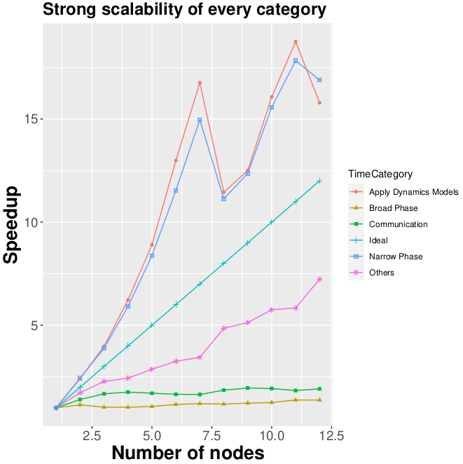
Let’s explain a little bit the strong scalability results, sit hows the time execution evolution according to the number of compute nodes, as well as the speedup plot. The R script loads and transform the data generated by XDEM and once obtains the time execution for the different phases, it creates a speedup plot for each category and focusing on the most relevant (the costliest categories). A heatmap of the efficiency accross different categories is included as well as a steamgraph of the proportion of execution time to observe the evolution and change in importance of the differente categories when more compute nodes are added.

Scalability for principal time categories

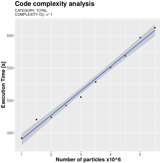
Another example, the complexity characterization identifies the complexity of the measured computing time for the principal categories as well as evolution graph of the time execution for the categories.
Besides it creates a heatmap for the scaling factor, checking as reference a linear increase, if it is scaling in a higher order it reveals a deficiency on the category.

Linear complexity for the apply dynamic models phase

Sadly it is time to say bye, but hey now XDEM has an additional tool that will help this software to keep track of the improvement over time, developers could attach it to XDEM continuous integration and even users could test with a little version of the original work to see which is the best decomposition or version for their project.

It has been a pleasure to be here with you kind readers and once again thanks to PRACE for this amazing opportunity :D.

My Summer of HPC has been centered around the FMM algorithm which has been roughly explained in a previous post. Studying its fundamentals and its sequential implementation was very interesting but it’s time to say goodbye. I will use this post to give a brief overview of my experience.

Getting started

The first task was to get familiar with FMM terminology and the basic principles that inspired it, some of which we’ve already covered. After that, we studied the layout of the octree that enables the reduced complexity that FMM offers. This was specially important because our goal was to come up with a MPI version in order to leverage a large amount of nodes.

Some difficulties such as dealing with their complex representation parametrized by many template parameters, or deciding how to distribute those octree nodes in a sensible manner motivated us to focus on the near field pass of the algorithm.

Speeding up the near field pass

The near field pass is pretty similar to a naive Coulomb solver, they only differ in that the near field pass focuses on a box and its close neighbours. Our first approach was to come up with the simplest implementation possible and measure how big the communication times grew as we scaled up in the number of nodes.

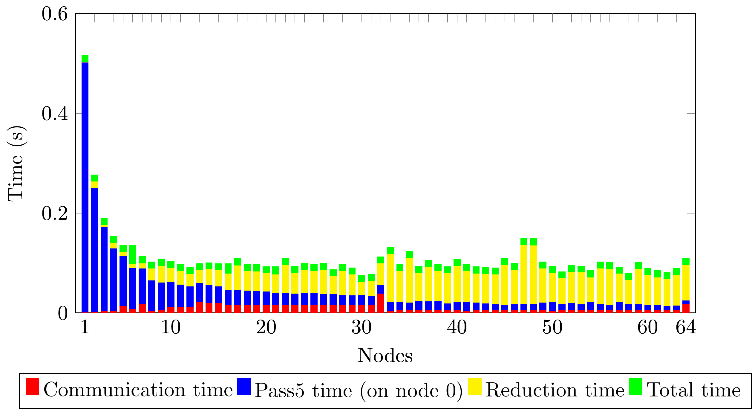
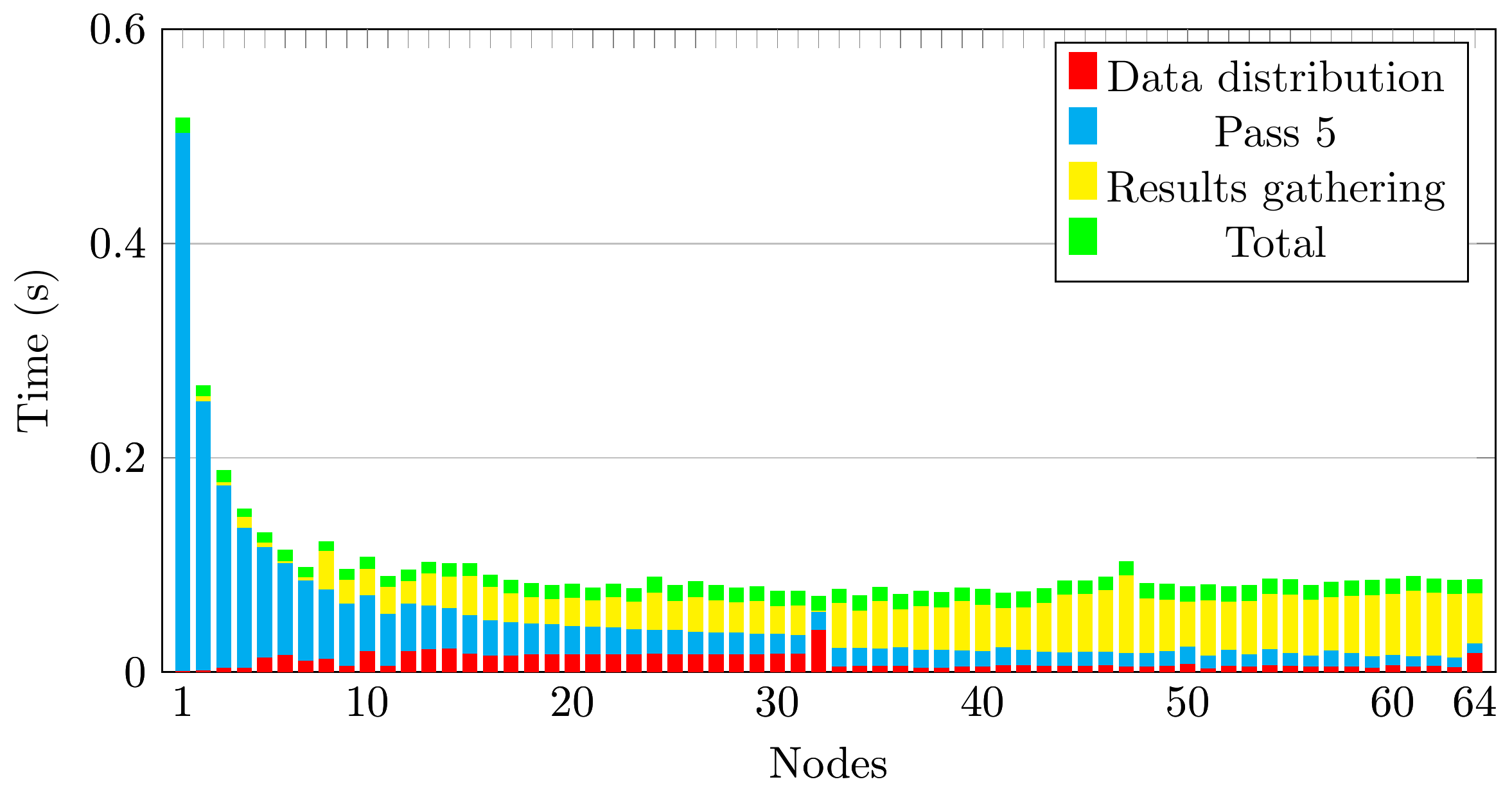
The results showed that the simplest schema performed surprisingly well on the data distribution part but extremely badly in the results collection. This indicates that broadcasting is very well optimized and that if we want to scale up in number of nodes we have to fix the reduction times.

At this point the hypothesis were three:

  • The message size is too big
  • Perhaps using a Reduce operation somehow chained the delays eventually adding up to a significant amount when the number of nodes grew.
  • There is a load imbalance in spite of the workload being highly homogeneous

Sadly every explanation I came up with proved to be wrong: there wasn’t load imbalance and greatly reducing message size and communicating it directly to the master node didn’t provide any significant speedup.

Conclusions

Our results show that our goal is not as easy as one might think at first. This is not good news but it also means that there is much work left to be done, and that should make you happy! Weird and complex problems leave you room to try crazy ideas and that is definitely fun.

On a personal note, Summer of HPC showed me the difference of tackling a very complex problem without a clear path versus solving a guided university assignment. This change can sometimes be frustrating but it is what it is. Doing research is difficult and you can’t expect to solve everything at first sight.

The experience has been great and much fun, and I would like to thank Ivo and the SoHPC team for making this possible.

Hello everyone! It’s been a while since my first post. And I look forward to giving you more detailed information about the data I’m working on.

How is the data structured?

There are multiple resources that can be used as data resources in the system analytics project. These are EAR, XALT, SLURM and Prometheus. I am working with Prometheus data. Prometheus is an open-source systems monitoring and alerting toolkit. The data coming from Prometheus contains a lot of information for HPC systems at the node level. Also, Prometheus creates a new datapoint about the node every 30 seconds. This means that we can get information about the nodes in the Lisa cluster every half minute. In order to obtain a uniform dataset, I worked on 6 days of data obtained from more than 200 CPU nodes. This means more than 4 million datapoints. Each datapoint contains 70 different features from file system usage to core temperatures and many more. This data, of course, was waiting for me in a compressed state in a database. (I am sharing a small section of the first datapoint for you below.) I needed to decompress this data first and then make it suitable for PCA analysis, which would allow us to extract useful features for our project.

id :  1
timestamp :  2022-07-08 05:16:17
node :  r11n1
node_arp_entries :  {'admin0': '15'}
node_boot_time_seconds :  1657200000.0
node_context_switches_total :  31588000.0
node_disk_io_now :  {'sda': '0'}
node_disk_read_bytes_total :  {'sda': '918531584'}
node_disk_writes_completed_total :  {'sda': '78263'}
node_disk_written_bytes_total :  {'sda': '6146845696'}
node_intr_total :  39498500.0
node_load1 :  0.0
node_load15 :  0.0
node_load5 :  0.0
node_memory_Active_bytes :  920846000.0
node_memory_Dirty_bytes :  0.0
node_memory_MemFree_bytes :  98187700000.0
node_memory_Percpu_bytes :  7012350.0
node_netstat_Icmp_InErrors :  0.0
node_netstat_Icmp_InMsgs :  57.0
node_netstat_Icmp_OutMsgs :  57.0
node_netstat_Tcp_InErrs :  0.0
node_netstat_Tcp_InSegs :  443546.0
node_netstat_Tcp_OutSegs :  435529.0
node_netstat_Tcp_RetransSegs :  2.0
node_netstat_Udp_InDatagrams :  1839.0
node_netstat_Udp_InErrors :  0.0
node_netstat_Udp_OutDatagrams :  3166.0
node_network_receive_bytes_total :  {'admin0': '2631816125', 'eno2': '0', 'lo': '3771950'}
node_network_receive_drop_total :  {'admin0': '0', 'eno2': '0', 'lo': '0'}
node_network_receive_multicast_total :  {'admin0': '2', 'eno2': '0', 'lo': '0'}
node_network_receive_packets_total :  {'admin0': '702717', 'eno2': '0', 'lo': '32833'}
node_network_transmit_bytes_total :  {'admin0': '145355117', 'eno2': '0', 'lo': '3771950'}
node_network_transmit_packets_total :  {'admin0': '408320', 'eno2': '0', 'lo': '32833'}
node_procs_blocked :  0.0
node_procs_running :  7.0
node_rapl_package_joules_total :  {'0': '52516.334246'}
node_thermal_zone_temp :  {'x86_pkg_temp_0': '26'}
node_time_seconds :  1657250000.0
node_udp_queues :  {'v4_rx': '0', 'v4_tx': '0', 'v6_rx': '0', 'v6_tx': '0'}
nvidia_gpu_duty_cycle :  None
nvidia_gpu_fanspeed_percent :  None
nvidia_gpu_memory_used_bytes :  None
nvidia_gpu_power_usage_milliwatts :  None
nvidia_gpu_temperature_celsius :  None
surfsara_ambient_temp :  24.0
surfsara_power_usage :  36.0
up :  1.0

Yes, this is the small portion of a single datapoint!

A bit of parallelization

In order to use the data in PCA analysis, all of the features had to be numerical values ​​and had to be normalized. First of all, I wrote a serial code for this. It took approximately 20 hours for this code to run in a database containing more than 4 million datapoints in total. But of course, our time is precious! So I parallelized the code and made it run 4x faster even on my local computer. (I’m going to be a little proud of myself here because I’m doing parallel programming for the first time :))

PCA Results

After pre-processing, I got 4787342 datapoints, each containing 74 features. Then I normalized this dataset and applied PCA. For ease of visualization in PCA, I primarily used 3 components. While doing this study, we expected to see some clusterings as a result of PCA, but the result has a linear structure. Could it be that it somehow made this inference even though we didn’t include the timestamps in our PCA analysis?

We also obtained other interesting results. Looking at the PCA components, we noticed that nothing about the file system is useful for explaining the data (i.e. almost), apart from that, things that produce output with similar units such as node1, node5 and node15 are almost equally important and rank higher when we order the components.

What is next?

Based on this study, we decided to continue with a single node, to get rid of some outliers with PCA analysis, and then to continue with a new dataset. I will share the details with you in my next post!

Welcome to my third and final blog post. At the end of the previous post, I briefly explained the goals of this project. I talked about making LQCD simulations to extract a pion mass and find an input quark mass that would give a pion mass value close to the experimental one. Of course, all of these are once again ambiguous so let me describe them step by step.

What Is Hadron Spectroscopy?

In QCD theory, almost every problem has to do with the calculation of various physical quantities using the path integral. However, those integrals are what perturbative techniques fail to calculate, which forces us to use the LQCD formalism. In our case, we will focus on a class of those problems called hadron spectroscopy. In these problems, we intend to find the mass of a hadron(e.g. a pion) based on specific input parameters.

The most essential input parameters are the gauge field configuration and the quark mass. To obtain a solution that converges with this of the path integral, we must carefully select a quark mass and conduct the same experiment with many different gauge configurations. Next, we can take the average of all outputs, which should lead to a relatively accurate solution depending on how well we chose those input parameters.

Path Towards Pion Mass Extraction

Since we discussed the necessary theoretical background, we can move forward with the procedure I followed to complete my project. Initially, I selected a quark mass equal to -0.01 and did simulations with many slightly different gauge configurations. Before you ask, yes the mass can be negative here! That happens due to an additive mass shift introduced during discretization, but it shouldn’t bother us. Also, I should clarify that all masses during the experiments are expressed in lattice units, which makes them dimensionless. That is yet another mathematical trick to make the calculations easier for the computer.

Upon completing those simulations, I extracted their pion correlators and calculated their average and standard error. A correlator is a function describing the relation of microscopic variables(e.g. spin) at different positions. The statistical observables we calculated are the key to the final step of this process. That step is to perform exponential fitting and acquire the pion mass. To achieve this, I utilized the tool called gnuplot. However, its pion mass error estimate was slightly inaccurate as it doesn’t consider the correlation among configurations. To remedy this, I replaced it by calculating the jackknife error, which is much more precise in such cases.

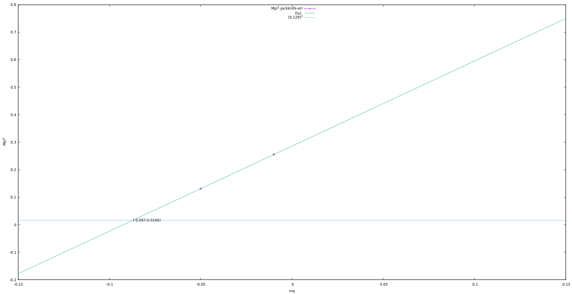
Figure 2: Graph with the line representing the relation of the pion mass square and quark mass. The horizontal blue line is at the desired pion mass square

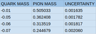
Finally, despite the already decent estimate of the pion mass value, I tried to get closer to the experimental value. That amounts to 135 MeV and translates into a lattice mass of 0.129. To this end, I exploited the approximately linear relation between the square of the pion mass and the quark mass to find an ideal target quark mass. I started by repeating the simulation with another quark mass equal to -0.05. Then, I created the line defined by the pairs we found, plugged in the desired pion mass square, and ended up with a quark mass of -0.087.

Final Results

Figure 3: Table with results extracted from experi-
ments with 4 different quark masses

Using such a low quark mass as -0.087 dramatically increased the complexity of the underlying linear systems, and the solvers in chromaform struggled to make the solutions converge. For this reason, the lowest mass I could try was equal to -0.07, though it still provided a satisfactory outcome as seen in Figure 3. If there was more time, I would probably search for the solution to this problem by modifying other aspects of the chromaform tool (e.g. the precision, max number of iterations of linear system solvers), but this can be an interesting future project!

A Journey That Came To An End

As all of us know, every good thing ends one day. Reaching the end of my journey with PRACE SoHPC, I reflect on the whole experience and consider it one of the most precious moments in my academic life. During the program, I learned many new things and broadened my horizons. It is an undeniable fact that PRACE SoHPC is a worthwhile experience, which I suggest to everyone.

P.S. Don’t forget to check the following video presentation we made with my colleague Christopher Kirwan about the project. Also, I strongly recommend checking out Christopher’s really interesting work about benchmarking with Kokkos API.

High Performance Quantum Fields Video Presentation

OpenFoam is a freely available open source package, widely used in CFD, facilitating the development of custom open source CFD NWT software for WSI problems, including modeling WEC. OpenFoam includes a large number of models, advanced gridding routines and parallelization options.

OpenFOAM’s broad user base is growing steadily, producing valuable features that complement the official version. Until now, it wasn’t clear how these developments would translate into official releases, benefiting from more users, maintenance, testing, and quality assurance.

OpenFoam capabilities.

OpenFOAM has a wide range of capabilities to simulate everything from turbulence in automotive aerodynamics, to combustion, chemical reactions, heat transfer, liquid sprays, films, and fires and firefighting in buildings. It includes tools for meshing in and around complex geometries, data processing and visualization, and more. To take full advantage of today’s multicore HPC infrastructures, almost all computations can be performed in parallel by default. Some of the available features in OpenFOAM are: Dynamic meshes, Numerical method, Linear system solvers, Parallel computing, etc.

Application of OpenFoam to permafrost modeling.

Why OpenFoam ?

It can be easily scripted, so the process can be fully automated. Once the enclosure is set up for the first time, changes in geometry or flow conditions can be quickly tested and compared with previous results. This can effectively optimize a wide variety of problems.

The processing speed is very good, and in combination with parallel programming options offered it can lead to far faster and better results.

Perhaps the most important feature, is that OpenFOAM® is 100% free, enabling this way everyone to have access to it.

Hello all! In my previous blog post, I described the procedure we follow to calculate the thermal conductivity of damaged Tungsten. This will be my final blog post, and I will share my results.

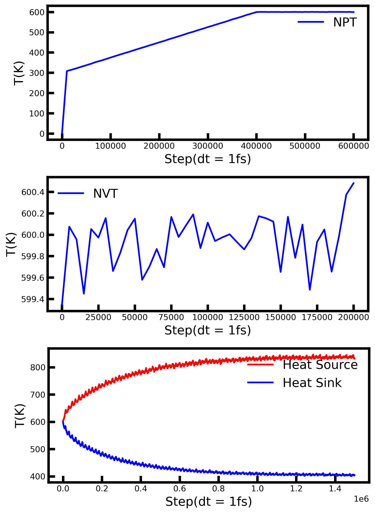
I investigated the thermal conductivity of Tungsten at 600K for several different damage levels. As prescribed in my previous blog post, each system was subject to CRA, NPT, NVT, and NVE processes. You can see the damaged part in the figure above. The red and blue atoms are interstitials and vacancies, respectively. The temperature changes of the system in NPT, NVT, and NVE are plotted with respect to molecular dynamics steps in the below:

As you can see from the last plot, the steady-state temperature gradient is established, and the temperature is nicely converged. Afterward, the temperature profile of the system is calculated and plotted as follows.

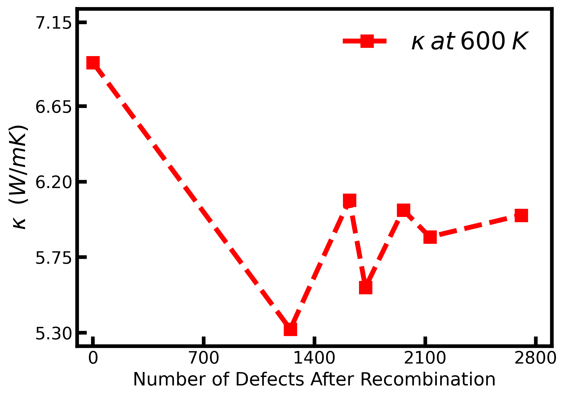
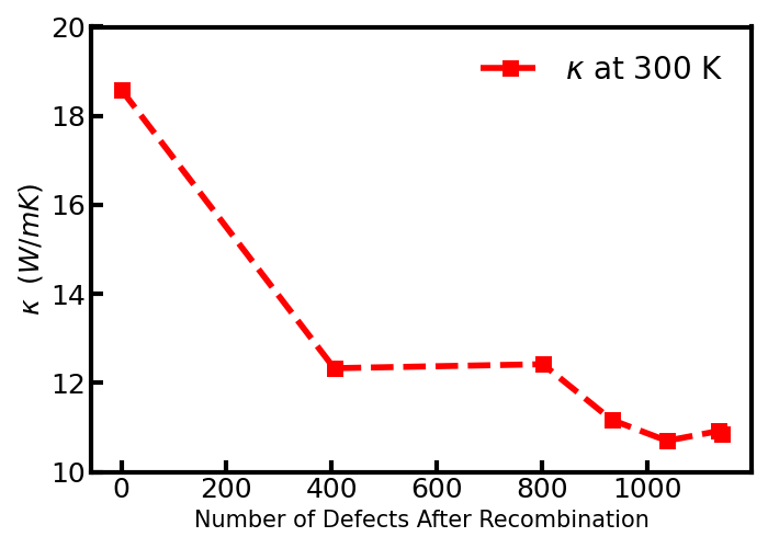
The same procedure is applied to other damage levels, and the resulting thermal conductivity is plotted with respect to the number of defects after recombination.

Although we can see that the thermal conductivity of the perfect system(no damage) is higher than the damaged systems, it is not clear to conclude a definite trend using the number of defects after recombination. Moreover, different defect types can form in the damaged part, which might differ in potential energy and geometry. This may lead to a difference in thermal conductivity for different damage levels. Therefore, the investigation can be broadened for other descriptors.

Participating in this program was a very rich experience for which I am very grateful. It was a pleasure knowing my mentors and Tanya, my project partner. Throughout the whole summer Dr. Gall helped us a lot in creating the models and instructed about what we should do. He knows a lot and he taught us more about Artificial Intelligence and Neural Networks. Dr. Pitoňák helped us in writing the report and making the video at the end of the project and gave us some good feedback.

I am very grateful to all of them for taking some time of their summer, which usually people use for vacations and other things, to be our mentors and for giving us such attention. Tanya and I were always helping each other and exchanging our progress and our results. I am glad she took the challenge of working on this project and that we could work together.

Although I knew some of the theory, I started the summer without having any practical experience with neural networks. I knew much about the concepts, but I had never used them in an actual project. Yet in this project, we used Neural Networks to create all our models, therefore I could immerse myself into the tools. After learning more about Keras and tensorflow I am much more confident and excited to work on future projects that use NNs to create models. In case you are interested in exploring what we did in detail, please check our final report. The video bellow is a presentation that we prepared to explain some of the work we developed.

Now I know better some of the practical challenges of NN and AI. In theory, these techniques seem very useful. Yet, when I was working with them I realized that they also offer some challenges. Finding a proper set of parameters is one of them. Sometimes there are so many parameters to tune that it is very difficult to explore all possible combinations. And once it is very difficult to tune all these parameters, it is also very unlikely to be certain that our model is the best and the tuning is optimal.

We also experienced how long the codes can take to run and how paralyzation can help. I had never faced these things before since the models I dealt with were much simpler and used much lesser data in the training process. Moreover, as we had access to different computers, it was interesting to see how the hardware can influence the time needed to run the codes. We got access to very impressive machines which was something I never had experienced before. Although I believe I couldn’t reach some of the initial goals, I am very satisfied with my overall experience with this project. Eight weeks can be short to learn about a new topic and also develop a project. Yet, I am impressed with everything I learned during this short period.

Even though we are finishing this project, I hope this will be only the end of a chapter for me. I believe that the techniques for molecule design that we learned will be the future of most chemical product engineering. And these techniques are just some of all the others there are available. As a chemical engineering student, I am very excited to deepen even further in the field. Certainly, the things that I learned during this summer will help me in my career, and it already influenced my master thesis.

For the students that are thinking about applying for the future of HPC, I totally recommend it. If anyone wants to learn more about what we did or more about my experience with Summer of HPC, or just wants to talk about something related to molecule engineering, feel free to contact me.

I want to thank everyone from PRACE for the awesome program that they offer during the summer. I also want to thank everyone that supported me during this journey, such as Isabela, Giulia, Daniela, Roberto, Juliana, and other friends and relatives. This is just the beginning of my journey through molecule engineering using computational tools. 

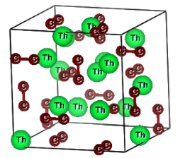
Thorium sesquicarbide (Th2C3) is a potential candidate as a nuclear fuel for generation IV advanced reactors. The microscopic structure of this compound is shown in the figure. Physicists call that cube unit cell of the material, i.e. the smallest portion of a crystal lattice that shows the pattern of the entire crystal: you can build your solid repeating this structure in all the three direction x,y,z.

Although a solid consists in billions and billions of atoms, the unit cell usually contains a few of them. For example, regarding Molybdenum (see previous blog) only 2 atoms are in the unit cell, for Palladium (see Mattia blog ) there are 4 of them. How can it be possible? How does a complicated problem reduce to a problem of few atoms? The answer is that there is a microscopic order, there are spatial symmetries that allow us to understand a solid starting from a small building block. However the unit cell of our compound is not so small, it contains 40 atoms (24 C and 16 Th). For this reason we need a supercomputer to perform all the calculations!

Electronic Properties

The first step to grasp the main features of this compound is to study how electrons behave, in particular how they make the bonds between the atoms and how the electronic charge is spatially distributed.

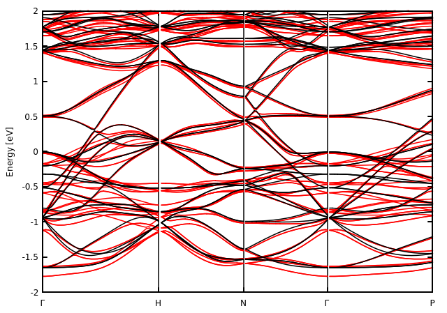
In the figure the so-called band structure of Th2C3 is reported. The vertical axis is the energy of the single electron with respect to a particular energy (Fermi energy). The horizontal axis is a quantum number defined from the periodicity of the crystal and related with the momenta of the electrons. The Fermi energy is set in such a way that it separates the filled states from the empty states. You have to imagine that in all the lines below 0 energy there are electrons while there are not above. So an electron near 0 requires an infinitesimal amount of energy to move in an empty state. This fact implies that the main properties of the material are determined on how many electrons are near the Fermi energy!

Lattice vibrations

Now that electronic problem is solved we can study how the ions move! The strategy is as follows:

  1. Find the equilibrium distance of the ions
  2. Make a little displacement of the ions to calculate the forces
  3. Use the periodicity to study only the problem in the unit cell

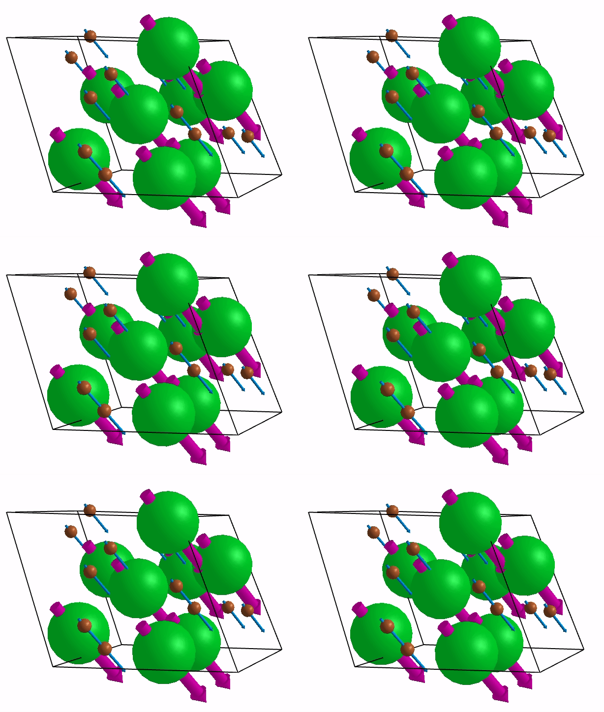
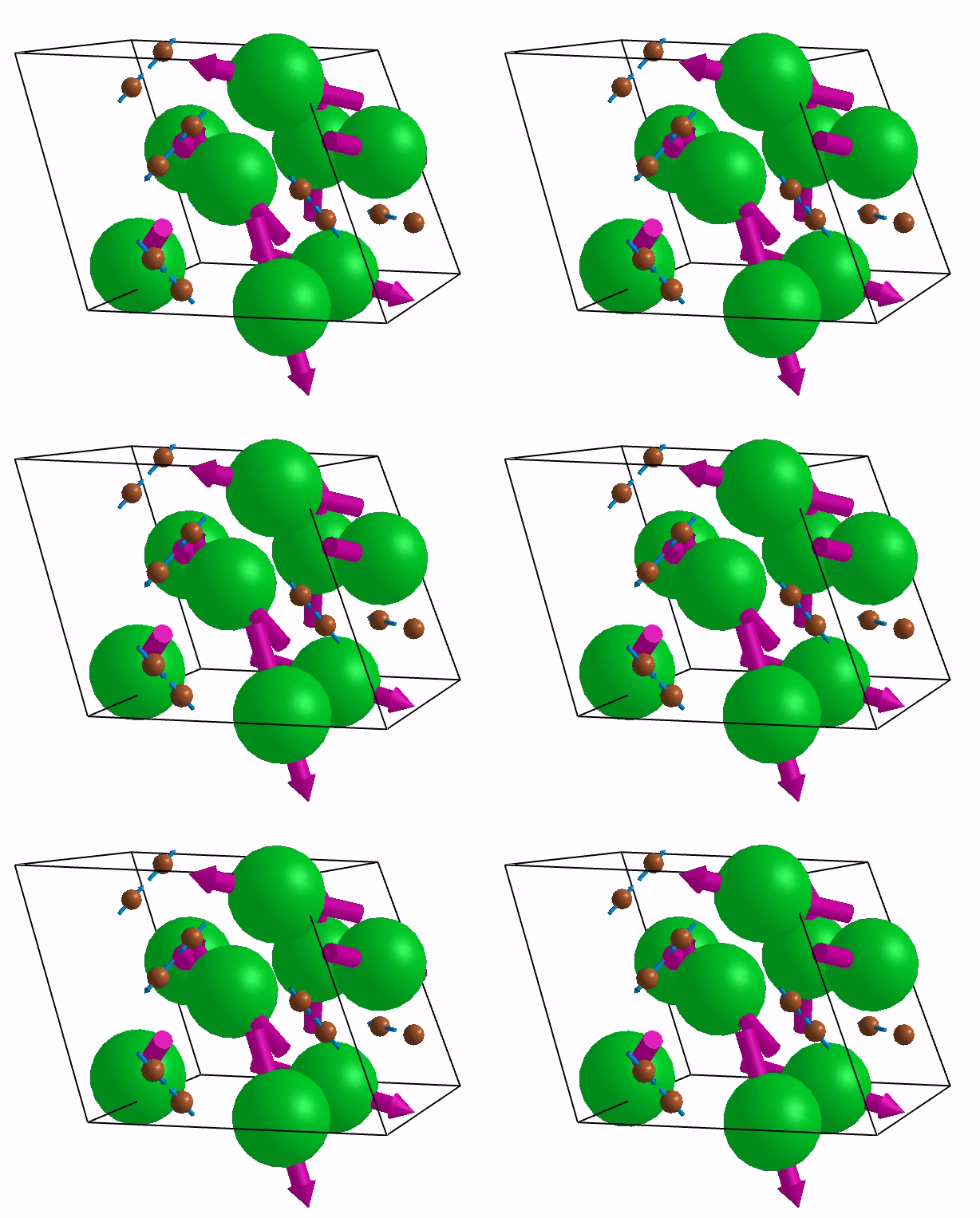
Below are shown some characteristic vibrations

These vibrations combined with electronic motion will determine thermal properties of the potential novel nuclear fuel!

Acknowledgement

I’m really grateful to every person that made my partecipation for the Summer of HPC 2021 possible. It is a fantastic experience that I would recommend to anyone interested in computational science and its applications. I hope you found my blog pages interesting and helpful to understand how we can deal with materials from a physical point of view.

In this blog post, I will share with you the ideas and goals behind the project 2203 “Neural networks in chemistry- Search for potential drugs for Covid-19“. As the title suggests, we will work on finding potential drugs for Covid-19 using artificial neural networks.

SARS-CoV-2

Severe Acute Respiratory Syndrome Coronavirus 2 (SARS-CoV-2) is a member of a large family of viruses called coronaviruses, first reported in Wuhan City, China, in December 2019. This virus had terminated all the activities around the world and had put a stop to everything for the past two years. It is the causative agent for COVID-19. Well, I believe there is not even a single human being who has not been affected, and in many cases (~582 million worldwide) infected by this virus. Although there are vaccines which provide great action against the virus, already developed by the pharmaceutical companies. There is still a risk of developing new mutations by the coronavirus producing even stronger variants on which the developed vaccines may not be able act, and hence fail to contain the spread of the future variants.

Development of vaccines

Now, when the spread of COVID-19 pandemic is reduced, all of us ask the same question, are we prepared for another pandemic? The best preparation against viruses is development of vaccines which can give long term protection to this generation and to the next generation. However, developing a vaccine is not easy, and require years of trials and tests of drugs, which are thought to potentially work as inhibitor on a disease or virus. Developing a drug is a long and cumbersome process where a big amount of capital and time is required.

Vaccines can help protect against certain diseases by imitating an infection. This type of imitation infection, helps teach the immune system how to fight off a future infection. While vaccines are the safest way to protect a person from a disease, no vaccine is perfect. It is possible to get a disease even when vaccinated, but the person is less likely to become seriously ill.

How vaccine development can be accelerated by using Artificial Intelligence (AI)?

Well, there are millions of drugs which may potentially save us from another pandemic. But the question is how to test such a large number of molecules. The answer to this question is modern computational tools such as artificial intelligence (AI), machine learning (ML), and neural networks (NNs). The development in advanced computational tools have connected many branches, and one such connection is among medical science, chemistry, and computer science. AI, NNs, and ML were constantly applied to predict the outbreak, and to calculate the molecular docking scores in search of COVID-19 inhibitors.

Artificial intelligence is a wide-branch of computer science that deals with the development of algorithms and techniques to solve complex problems which typically require human intelligence. Modern approaches in AI are focused more on machine learning (ML) and deep learning (DL). In simple words, ML is defined as the capability of a machine to identify patterns from the available databases, through a learning process. An advanced version of ML is DL which consist of developing algorithms to create artificial neural networks (ANNs) that can learn a process just like neurons of human brain.

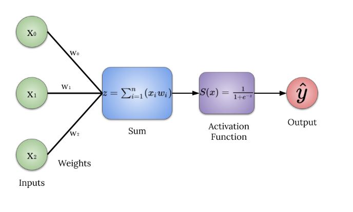
An example of a neural network model.

ANNs is a group of artificial neurons that takes the available data as input, passes it through one or more hidden layers where a weight is applied to the inputs, and is directed through an activation function. The activation function performs the non-linear transformation on the inputs and send the predictions to the next layer, and the process is repeated for the total number of epochs. The predictions are compared with the outputs of the problem to see the goodness of the fit. Often, mean squared error is computed between the predictions and the outputs to check the efficiency of the training. The training procedure depends on a number of parameters namely, number of neurons, number of hidden layers, learning rate, activation function, optimizer, bias and weights.

Goals of the Project

The main aim of the project is to find potential drugs against the SARS-CoV-2 virus using Neural Networks and Molecule Descriptors. The protein responsible for the virus replication, 3CL pro SARS-CoV-2 (6WQF) is the targeted protein under this study. The Python libraries TensorFlow and Keras will be utilized to develop neural network models, and Dscribe library will describe the input molecules using its available molecular descriptors. We will look for correlations between the molecular structures of the investigated chemical compounds, and their computed docking scores from the neural network models. The potential drugs based on the docking scores will open new pathways towards the future research in search of potential drugs against coronaviruses and would help in preventing any future outbreaks.

Thank you for reading this blog post. Stay tuned for the final blog post which will contain some interesting results from our work, and who knows maybe we will be able to find a permanent vaccine against coronavirus. If you feel fascinated by the subject and would like to know more about the process of developing drugs, then read this article from a previous work. Feel free to ask any question or write your questions in the comment box below. See you in the final blog post!

In my last update, I mentioned that I applied PCA for all datapoints and the results. But I have hidden an important detail for this post 😉 When we added the explained variance percentages as a result of PCA, we could only approach 40%. This means that we were only able to obtain 40% of the information about all datapoints.

Less Data, More Components

Then, in order to get more successful results, we decided to shrink the dataset we applied PCA and increase the number of components until the explained variance percentage increased. Thus, I started working on a dataset containing nearly 200 thousand datapoints containing information about 10 nodes. We chose these nodes according to their CPU usage rates. We tried to select the nodes with the most job submissions within the selected 6 days.

Afterwards, I increased the number of components one by one and made PCA analysis. As a result, we reached a 98% variance explained using 15 components.

Outlier Detection by PCA

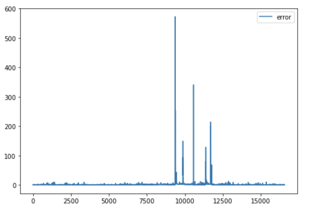
Error rates for one of the nodes. The nodes has 16 thousand datapoints which are on x-axis, while y-axis shows the error rate.

After that, we used 15 components in all PCA analyzes we did. We decided to clean up the dataset a bit with the help of PCA analysis. For this, we used the reverse transforms of the principal components, which we obtained as a result of the PCA analysis. Then, using the distance between these values and we removed some of the outliers from the dataset. While doing this, we set the maximum error rate as 5, in this way, we kept 95% of the data in the dataset and eliminated 5%.

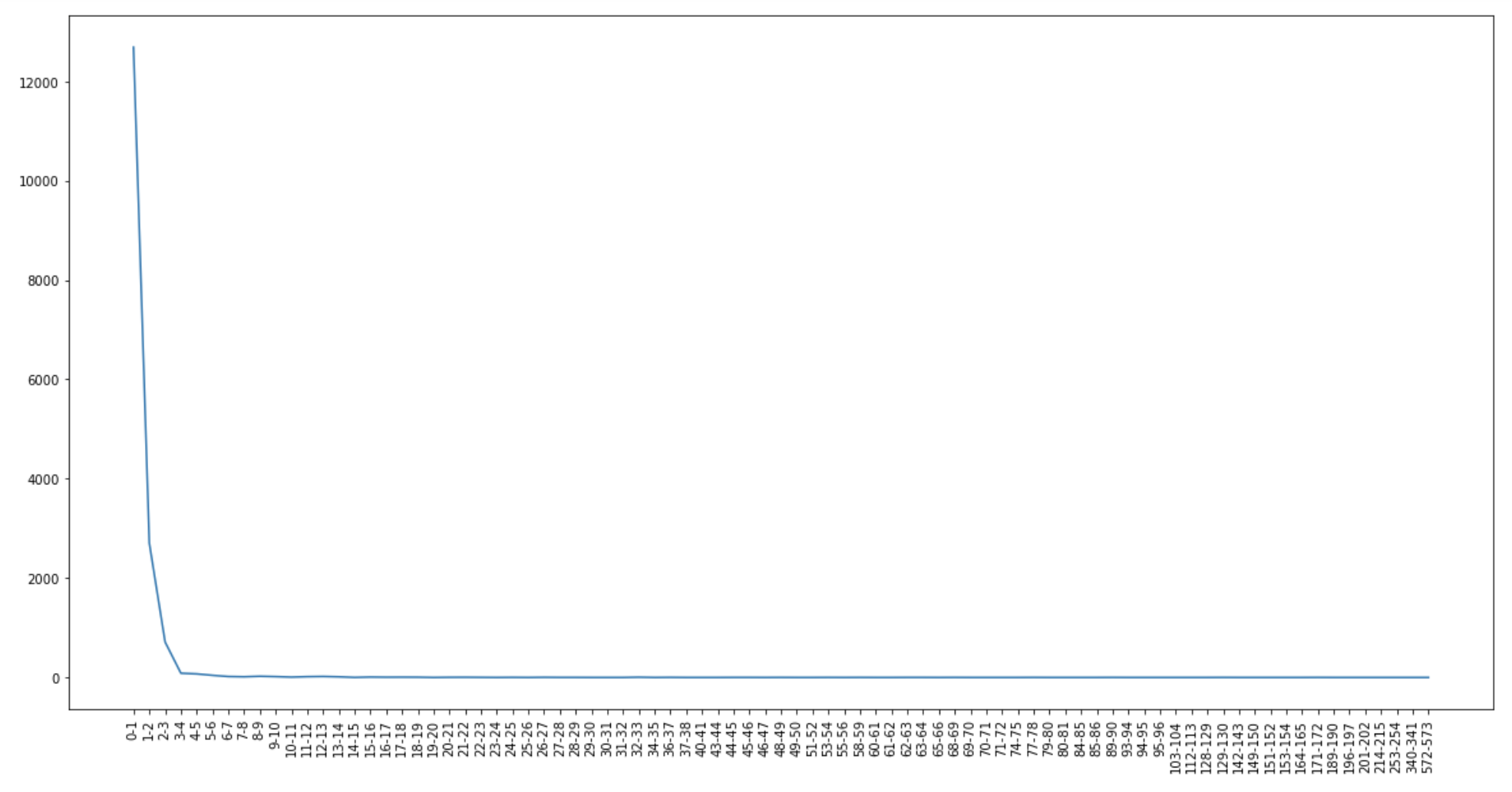
Count of error rates in certain ranges. Mostly datapoints have error between 0-1 or 1-2. The x-axis shows the error ranges, while y-axis shows count of datapoints that have error rate between that interval.

Didn’t We Already Find the Outliers?

But of course, the question here is why did we clean this dataset? Wasn’t our goal to find outliers anyway? Yes, our goal is to find an outlier. But our plan for doing this is as follows: Let’s train a machine learning method on timeseries data and that model can predict the features in the next step. We will use this clean dataset to train this model. Next, we will find the anomaly using the model’s predictions.

Next Step

We’ve come to the coolest part of the project! Selecting a machine learning model and training it with this dataset that we cleaned. If you’re waiting for GPUs to mess with this, see you in the next post!

As I explained both the methods used as well as the field of application of my project in my last two blog posts, I now want to gather all the information and finally describe which simulations were carried out by my colleague Arda Erbasan and me.


Setup

How to calculate thermal conductivity using molecular dynamics?

Using the definition of Wikipedia: The thermal conductivity of a material is a measure of its ability to conduct heat. For a given material it can be computed with the aid of Fourier’s law q = -kappa ⋅ ∇T where q is is the heat flux and ∇T describes a spatial temperature gradient. Thus knowing q and ∇T enables us to calculate the thermal conductivity kappa. One possible way of doing so, is to define two distinct regions in the simulation box and add/subtract the same amount of energy to/from the two regions respectively establishing a known heat flux q and a temperature gradient ∇T between the resulting hot and cold region[1,2].

Sketch of the simulated system.

In our specific case we created a simulation box of cuboid shape and dimensions of ~ 158 x 15.8 x 15.8 nm consisting of 2.5 Million (!) individual atoms. A region (labeled ‘A’ and ‘B’ in the sketch) was defined at one quarter as well as at three quarters of the total length. Right in the middle between these two regions, another distinct region (labeled ‘C’) was defined. Here, the thermal conductivity is calculated later. Before the temperature gradient is established, defects, as caused by high irradiation, are created in region ‘C’. For this purpose, a method is used which I will describe shortly.

Furthermore, the entire system is now heated in several stages to a desired target temperature. Only then, energy is added/subtracted from regions ‘A’ and ‘B’ respectively and thus the difference in temperature is generated. Since we are using periodic boundary conditions, a second heat flux will also form, going through the boundaries of the simulation box. However, due to the symmetry of the system, this is accounted for by dividing the heat flux q by a factor of 2.

How to simulate radiation damage using molecular dynamics?

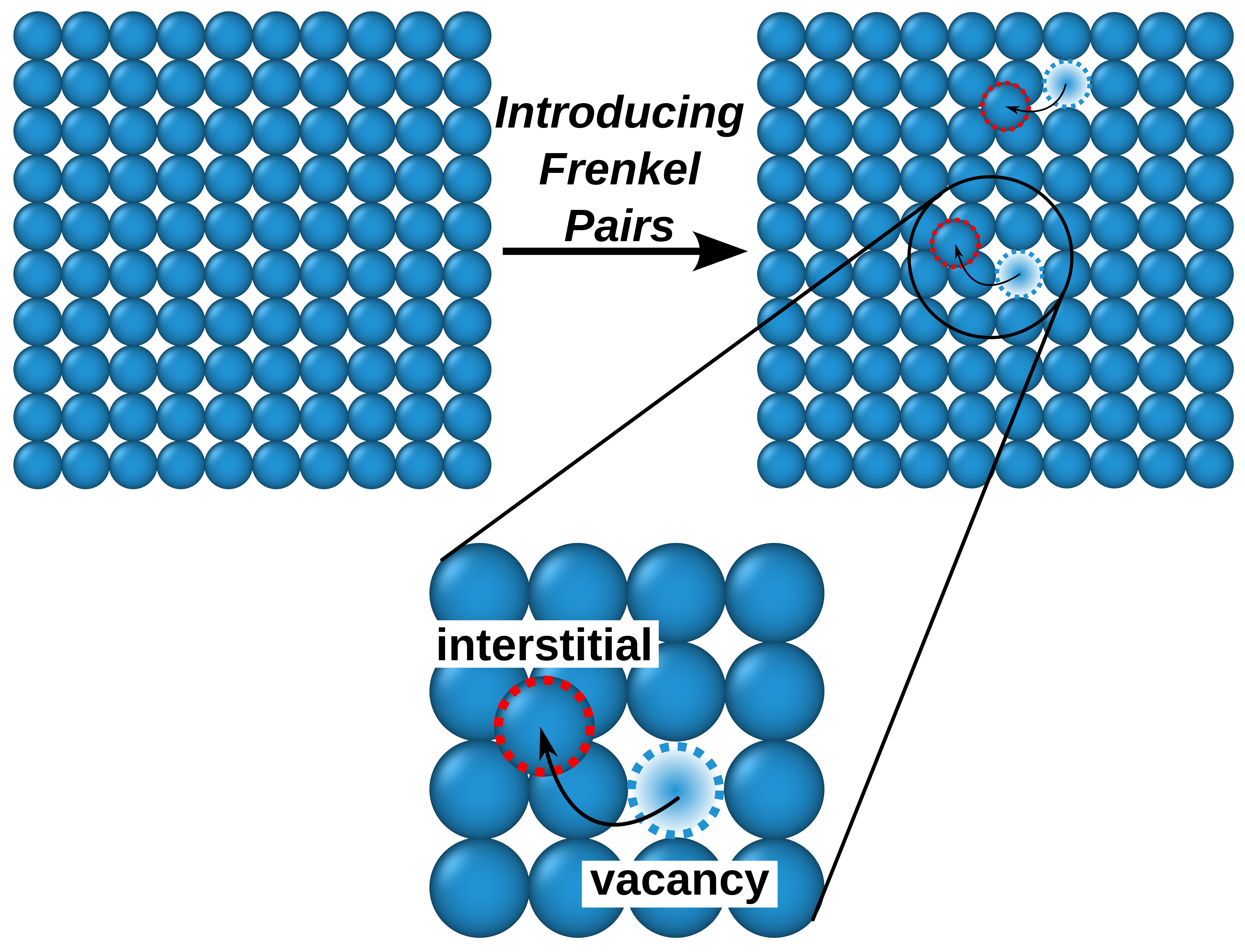
Since we are interested in the thermal conductivity of irradiated tungsten, we use an algorithm called “creation-relaxation algorithm” – CRA[3] for short – to simulate radiation damage inside the metal at relatively low computational cost.  In it’s essence, this method first displaces a random atom in the crystal to a new random position and then minimizes the energy of the new configuration (relaxation step) thus introducing pairs of vacancies and interstitial atoms – also called “Frenkel pairs”. This procedure is repeated until a desired level of damage is reached – as measured by the amount of displaced atoms. As mentioned before, the system undergoes a heating procedure after damage is created but before the thermal conductivity is measured. During this thermalization procedure, some of the created Frenkel pairs recombine and thus vanish.

The image below shows examples of said defects. Red are interstitial atoms, forming extended defect clusters and blue are vacancies. The green and pink lines indicate dislocation loops, a special type of defect structure, about which I will not explain in detail here.

Observed defects in a tungsten system using the CRA method.

Results

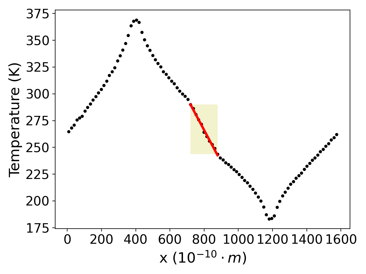
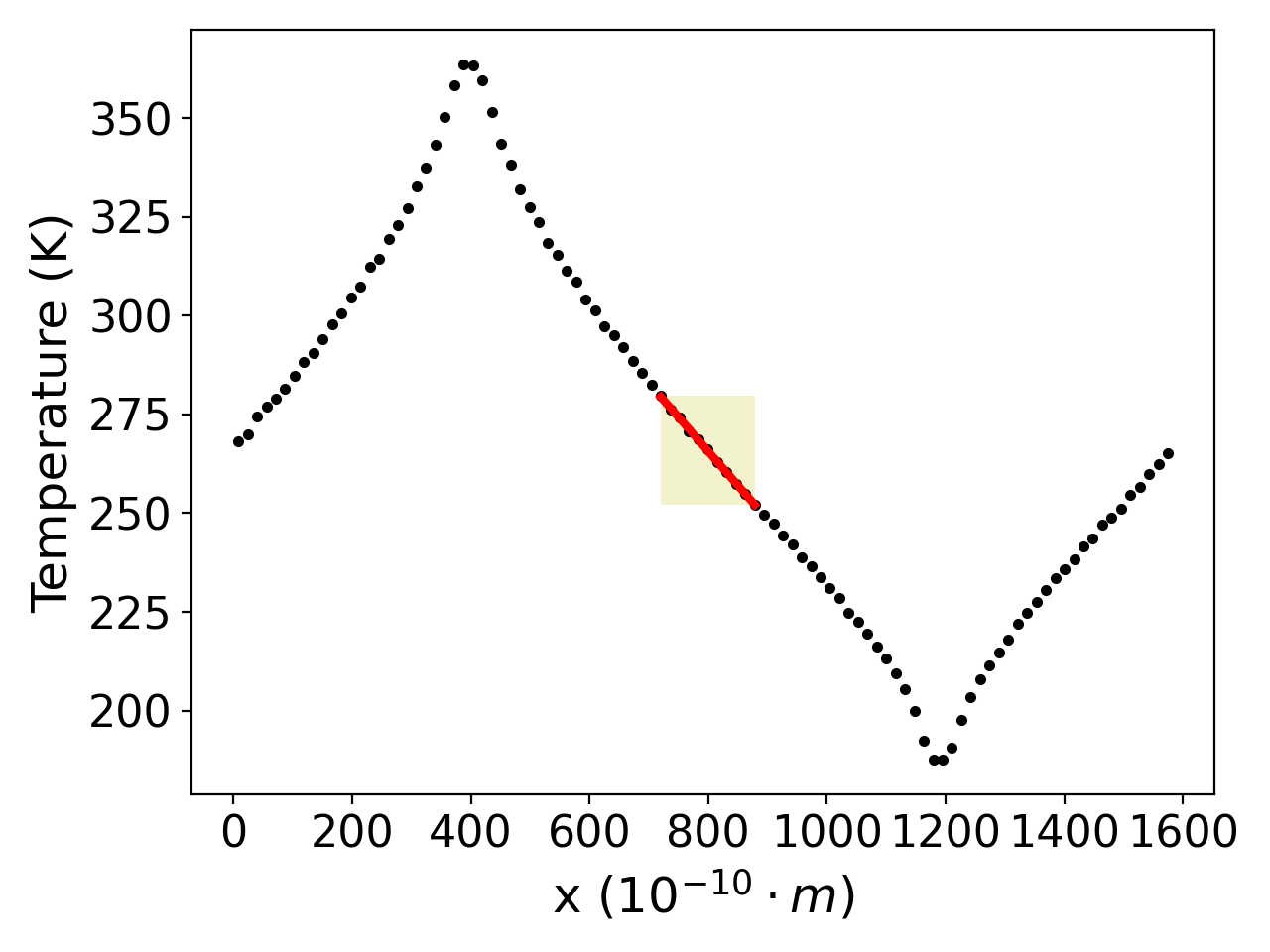
The following plots display the temperature profile of an undamaged system on the left and a damaged system – with 1038 final defects after recombination – on the right, both at a temperature of 300 K. The temperature profile was computed in the direction of the imposed heat flux.

The interesting part for us is located in the middle, which corresponds to the middle 10% of the system as described on the previous slide. In the undamaged system, we observe a smooth temperature gradient from the hot to the cold region. In contrast, in the damaged system, a clear change in the slope of the temperature gradient can be seen. This indicates poorer thermal conductivity: The perfect system exhibits a thermal conductivity of 18.59 Watts per Meter-Kelvin while the damaged system has a thermal conductivity of only 10.7 Watts per Meter-Kelvin.

To better quantify this behavior, we analyzed the trend in thermal conductivity with respect to the overall damage of the system as measured by the final number of defects. As can be seen, an increase in the number of defects comes with a decrease of thermal conductivity. We also observed some deviations from the main trend – possibly due to the statistical nature of the simulations.

Thermal conductivity for different levels of damage.

A few remarks on computational effort

Using 10 compute nodes of MareNostrum4 each one equipped with 2 sockets Intel Xeon Platinum 8160 CPU with 24 cores each @ 2.10GHz the whole simulation of a 2.5 Million atom system for a total of over 1 Million time steps was completed in less than 3 hours.


Conclusion

To wrap up, using this simulation setup we were able to observe a decrease in thermal conductivity of irradiated tungsten as compared to a perfect tungsten system. Although further tests would be beneficial, not least to counteract the statistical nature of this method and to make more robust statements, these results are already very interesting as they clearly show how certain properties of tungsten, in this case the thermal conductivity, change under radiation load in a fusion reactor. This must, of course, be taken into account in the construction of future reactors and especially in the service life of wall elements and plasma-facing components. In this sense, the molecular dynamics simulations can be a first step towards a full-scale simulation of a fusion reactor.


References:
[1] Ikeshoji and Hafskjold, Molecular Physics, 81, 251-261 (1994).
[2] Wirnsberger, Frenkel, and Dellago, J Chem Phys, 143, 124104 (2015).
[3] P. M. Derlet and S. L. Dudarev, PHYSICAL REVIEW MATERIALS 4, 023605 (2020).

What is LSTM and why did we choose to use LSTM?

LSTM, or long-short term memory, is an artificial neural network model that can process data sequences. This is especially important for time series prediction, as LSTMs can remember long term observations. But since LSTMs are powerful models, we have to be careful when using the model. The given input and hyperparameters are very important. Therefore, it is necessary not to forget the possibility of not getting proper results even though the problem is the time series.

What I want to do with LSTM?

We have a dataset of 10 nodes’ Prometheus information cleared of outliers. Using this dataset, we want to make predictions with the help of LSTM, and to find anomalies in the system with the predictions we made.

Some of the questions we will face when making predictions with LSTM will be: How much historical data will we feed and how far away do we want to predict data? Is the dataset we have enough, will it cause overfitting? What should the hidden layer size be? What should our batch size be?

Here we first decided to predict only cpu usage. Because cpu usage usually follows a trend. So if it’s high in the current step, it will likely be high in the next step. Therefore, we primarily focused on this feature only to get relatively good accuracy.

Look at the Results!

And when we started our experiments, we only used the data of one node (the node with the most job run). Since this node was in constant use, it also included unexpected spikes. So it was a node that was not easy to predict. Afterwards, we tried to obtain the next 50 predictions by feeding the last 100 observations. We fed the entire train dataset for each epoch and trained approximately 200 epochs of LSTM.

Of course, the first results we got were not quite as we wanted. But among the many parameters we can change, which one should we start with?

First of all, we stopped feeding the last 100 data, because it still showed all the information of the node in the last 50 minutes, we reduced it to 8. We also started estimating the next second CPU usage to reduce the likelihood of the model overfitting. We experimented with changing our hidden layer size from 2 to 64. We started using dataloaders. We got results by changing our batch size from 16 to 1024. Again, to prevent overfitting, we added dropouts, applied dropouts at different rates, and experimented.

In short, we did experiments using different hyperparameters hundreds of times and finally we reached some baseline results :))

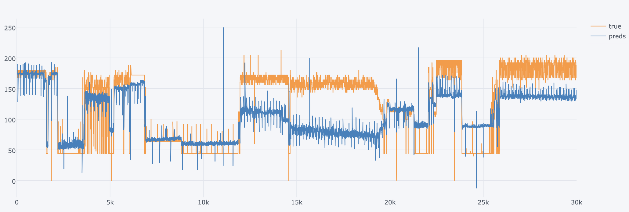
The baseline results of LSTM on test dataset

Looking at the results, we see that the model is able to predict up and down trends in CPU usage. This is good news for us! So is there still room for improvement? I wonder if we can achieve this accuracy by using less features? Is it possible to get better test loss results by changing the fed sequence length or playing with hidden size? Wait for the next post for the answers to these questions!

In my previous blog post, I mentioned using classical molecular dynamics implemented in LAMMPS. Let’s dig a little into the procedure and learn how we calculate the thermal conductivity of damaged Tungsten.

Although there are a massive collection of things you can do with LAMMPS, our procedure involve three main steps, and these are:

  1. Introducing damage to simulate irradiated Tungsten / Creation-Relaxation Algorithm(CRA)

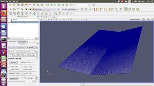
How would you imagine a neutron bombardment to a material? Neutrons hit the surface, and the impact will spread through the material, displacing the atoms from their natural sites to a higher energy position. This is one of the ways to simulate the damage. However, the time required to observe the damage on a broader scale and for high doses is pretty lengthy. This also means that the use of computational resources is extremely high. Luckily, Creation-Relaxation Algorithm is a shortcut to simulate high-dose damage swiftly. In this iterative method, randomly selected atoms are displaced such that there is a vacancy in the initial position of the atom and an interstitial(Figure 1). These pairs are also called Frenkel pairs. Then, energy minimization is performed, and the atoms settle to their new positions. Finally, these steps are repeated until the desired damage level is reached. In our study, we applied damage to the middle 10% of the simulation box(Figure-2).

Figure 1 Illustration of Frenkel Pairs

2. Thermally equilibrating the system:

Since we will investigate the thermal conductivity, it’s time to introduce the temperature and pressure factor to our damaged system.

  • Isothermal-Isobaric Ensemble (NPT): In this thermodynamical ensemble keeping the number of particles(N), pressure(P), and temperature(T) constant, we increase the temperature of the system to the desired value. While this happens, the volume of the simulation box changes until it converges to a value for a given pressure and temperature.
  • Canonical Ensemble (NVT): After obtaining the well converged system from the results of NPT, we put the system into canonical ensemble where the number of particles(N), volume(V), and temperature(T) are constant. The main reason we apply this step after thermally equilibrating the system is to obtain a statistically probable state of the system under given conditions. 
  • Introducing temperature gradient in microcanonical ensemble(NVE): In this step, we construct a heat source(hot region) and heat sink(cold region) within the simulation box. This is achieved by withdrawing kinetic energy from the heat sink and supplying the same amount of kinetic energy to the heat source(Figure 2). To obtain a steady state temperature gradient between “hot” and “cold” regions, we let the energy be distributed along the simulation box in microcanonical ensemble. As you can interpret the constants of the system from its abbreviation, the number of particles(N), volume(V), and total energy of the system(E) are held constant.
Figure 2 Illustration of the Simulation Box

In step-2 and step-3, the interstitial atoms can fall into the vacant sites, or new atoms can leave their sites and create a Frenkel pair. You can see an animation in the featuring image taken from one of our calculations in step-3. If you want to learn more about how we calculate thermal conductivity, you can check out this blog post from Paolo, who was one of the last year’s participants in the project!

In my final blog post, I will share my results with you!

OpenFOAM is a widely used CFD toolbox in academia and industry. It is also used to solve HPC problems related to fluid dynamics. However, some problems can take too much time to execute. For computation-heavy problems, parallel programming can dramatically reduce the computation time.

OpenFOAM has native support for parallel programming with MPI but writing parallel programs in OpenFOAM is not the same as writing parallel programs with MPI.

It was difficult for me to learn parallel programming in OpenFOAM at the beginning of the SoHPC. This kind of blog could have helped me so much. So, that is why I decided to write this blog.

Disclaimer

Most of the information presented here is derived from my experience during the Summer of HPC project which is developing a parallel pre-processing utility in OpenFOAM. I am neither expert in parallel programming nor OpenFOAM. Therefore, please use these examples at your own risk.

Prerequisites

The compiled version of OpenFOAM-dev (v2106 is used in this blog but unless it is too old, you can use any version)
OpenMPI (for installation you can refer to this article)
Knowledge of how to compile a program in OpenFOAM using wmake

A Basic Hello World

Let’s write a basic hello world program and run it in parallel. The details of compiling the program are not given here. You can look at other OpenFOAM programs’ Make directory to have an idea of how to compile your program.

When we run our program, we have to provide an extra argument to let the compiler know that this run is not a serial run. Therefore, we have to include setRootCase.H file inside the main function to set up the basic command-line arguments to provide the program.

#include "setRootCase.H"

The reason why we add this line inside the main function is that this header file is constructed from the arguments (int argc, char* argv[]) in the main function.

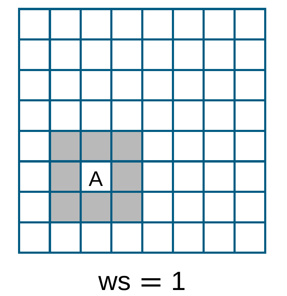
By default, our program searches for processor directories and if it does not find any directory like processor2, it throws an error saying that it could not find this directory. If you do not want your program to search existing processor directories, you can disable this behavior by:

argList::noCheckProcessorDirectories();

If you want to disable this behavior, add this line above the line where you include setRootCase.H file.

So far so good. Now, the final step is to print the message to the console:

Pout<< "Hello from process " << Pstream::myProcNo() << endl;

In serial applications, Info is used for printing messages to the console. For parallel application, Pout is used. However, Info can still be used in parallel applications. Keep in mind that Info only prints the message in the master process.

This is what the final program looks like:

#include "fvCFD.H"

int main(int argc, char* argv[]) {
    argList::noCheckProcessorDirectories();
    #include "setRootCase.H"
    if (!Pstream::parRun())
    {
        FatalErrorInFunction
            << ": This utility can only be run parallel"
            << exit(FatalError);
    }
    Pout<< "Hello from process " << Pstream::myProcNo() << endl;
}

After you compile the code, you can run this program by:

mpirun -np <number-of-proc> <program-name>

I also added a check to make sure the program is run only in parallel. If someone tries to run it in serial, it will complain and throw an error.

Pstream Class and Collective Communication

As you can see from the above example, we did not use MPI routines in our program. OpenFOAM provides a wrapper class called Pstream. We can use this class for the inter-processor communications stream.

For instance, gathering information from other processes is a common task. For that, we can use Pstream class’ gather method:

labelList data(10, Pstream::myProcNo() + 1);

Pstream::gather(data, multiplyOp<labelList>());
if (Pstream::master())
{
    Pout << data << endl;
}
Pstream::scatter(data);

Pout << data << endl;

Above code block gathers labelList data from each process multiplies these lists and scatters the result to all processes.

There are many binary operations that can make collective communication effective. Here are some of the available binary operations on labelList data structure:

  • plusOp<labelList>()
  • minusOp<labelList>()
  • divideOp<labelList>()
  • minOp<labelList>()
  • maxOp<labelList>()

For the full list, please checkout ops.H file.

There are many other methods that Pstream class provides. You can check out Pstream.H file for the rest.

One of the problems I faced during this summer was this problem:

You have 8 cells of a computational domain and split the domain into 4 partitions. The first two numbers of the list are calculated on processor 0, the second two numbers of the list are calculated on processor 1, etc. The data looks like this:

processor 0: 8 (0 0 0 0 0 0 0 0)
processor 1: 8 (0 0 1 1 0 0 0 0)
processor 2: 8 (0 0 0 0 2 2 0 0)
processor 3: 8 (0 0 0 0 0 0 3 3)

How can you gather the list from all processors like 8 (0 0 1 1 2 2 3 3)?

The numbers are arbitrary but explain my problem very well. Here is the code snippet that solved my problem:

#include "PstreamReduceOps.H"

// for setting up the data
labelList data(8, 0);
data[Pstream::myProcNo() * 2] = Pstream::myProcNo();
data[Pstream::myProcNo() * 2 + 1] = Pstream::myProcNo();

reduce(data, sumOp<labelList>());
Pout << data << endl;

Point-to-Point Communication

Let me illustrate this topic with an example. Below you can see an example of point-to-point communication:

labelList data(Pstream::nProcs(), Pstream::myProcNo() * 10);
// -1 indicates empty
labelList recvData(Pstream::nProcs(), -1);

// send
if (Pstream::myProcNo() < Pstream::nProcs() / 2)
{
    label destination = Pstream::nProcs() - (Pstream::myProcNo() + 1);
    OPstream send(Pstream::commsTypes::blocking, destination);

    send << data;
}
// receive
else
{
    label target = Pstream::nProcs() - (Pstream::myProcNo() + 1);
    IPstream recv(Pstream::commsTypes::blocking, target);
    recv >> recvData;
    
}
Pout << recvData << endl;

Assume the number of processes used in this program is 10. In that case, process 0 communicates with process 9, process 1 communicates with process 8, etc. Receiving processes hold their data in another variable called recvData. In the end, each process prints its data to the console. As you can see above, to send or receive data you have to create OPstream or IPstream objects, respectively. You can consider these as MPI_Send and MPI_Recv. In order to avoid deadlocks, make sure that the number of OPstream is equal to the number of IPstream.

Conclusion

There are many things that can be done with Pstream. However, it is not possible to fit everything into one post. If you think something is wrong or you want extra examples, please let me know in the comments.

Thank you for reading.
In my project “Heat transport in novel nuclear fuels“, as mentioned in the previous blogs, it is studied the influence of carbon atoms in uranium and thorium compounds in their heat transport. So, in the last weeks of this Summer of HPC, I had the opportunity to put my hands on a possible novel nuclear fuel, U2C3. You can see the complicated structure of this crystals in the feature image of this blog. There are 40 atoms in the most simple cube that you can cut from the entire solid! So many atoms and a big supercomputer that can handle them! To do all the calculations I used the Barbora cluster in the IT4I supercomputing center in Ostrava. It consist of 201 compute nodes, totaling more than 7000 compute cores!

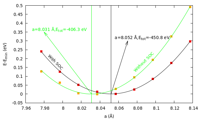
To calculate the electronic properties, I first found the equilibrium distance of the ions, the so called lattice parameter. The procedure to find it is quite intuitive. You fix the volume of your solid, you ran the VASP code that calculates the total energy of the system, then you “press” or “dilate” the structure, you repeat the calculation and so on. At the end you will find an energy-volume curve. The minimum of this curve is exactly the position in which the crystal is at the equilibrium.

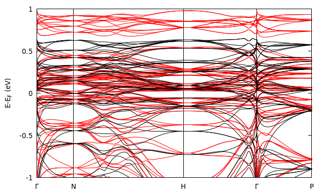
An important feature of uranium atoms is their big charge so electrons around them can move very fast! Therefore relativistic effects (the so-called Spin-Orbit Coupling) on this compound may not be negligible. Luckily, in the VASP module, there is the possibility to take it into account (with the effect of slowing down the calculations). Having this in mind I calculated the electronic properties with and without this correction. What it is showed in the figure below is the electronic band structure. What is it? To understand that we have to think about how do we solve the the crystal structure. Since we are dealing with microscopic matter, quantum mechanics is needed. At the end we have to solve a Schrodinger-like equation that will eventually give as all the quantized energy of the system. Another feature that a crystal has is the ordered structure. Just from this fact it exist a relation between the momenta of the electrons and the periodicity of the solid. So, at the end, what are these bands? Simply the plot of the quantized energies over this sort of momenta.

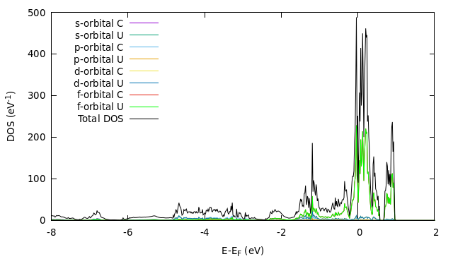
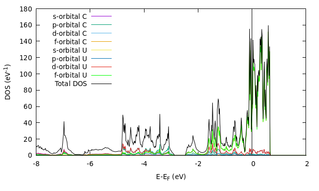
As you can see both from the bands and from the energy-volume curve, the SOC is sensibly not negligible! We cannot exclude the SOC in further calculation and unfortunately it will slow down the codes. But problems never ends! Uranium has also a magnetic moment and we have to include it. To understand thermal properties, we need to ask: how many electron states are available for the heat transport? Let’s look at the Density of States, more specifically at the projected DOS. This will tell us what kind of electrons are involved in the thermal conductivity. As you can see in the graph below, mainly localized electrons (f-orbitals are localized) from uranium are available (only electrons around zero energy matters!). Further calculations can be done to compute phonon and thermal properties.

And now we are at the conclusion of this SoHPC. I really enjoyed this experience and I hope that I have passed on to you my passion for physics and computational science. Goodbye everyone, it’s been a pleasure!

Satellite-derived bathymetry using machine learning and optimal Sentinel-2 imagery in South-West Flo

Check out my last results with machine learning.
In my previous posts I introduced my work mapping the seabed in the Calabrian Sea. Just a few weeks ago I succeed mapping this Sea using one algorithm that uses band ratios to estimate depth. I shared you this map in my last blog and I promised you that I would start working on the same but using machine learning (ML) and I will show you the results. So, here you have the results and a briefly explanation of the computational process.

The process

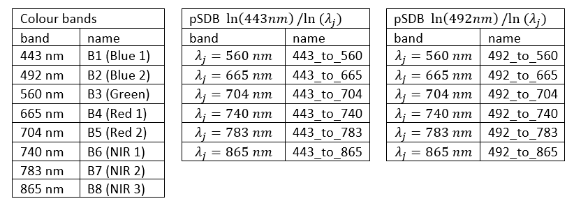
I worked in the same area covering bathymetry up to 20 meters. I used only the 80% of one satellite image to train the regressor and I tested the model with other images. But this time I considered other variables (See figure 1) such  colour bands and pSDB ratios.

List of features used to train the ML model.

Between all ML methods I chose Random Forest (RF) because it´s a popular method to estimate the importance of the input variables. I did several test using different combination of features and I found out that the most important features are the colour bands blue, red, green and near infrared, and the most important ratios are those between blue and green, blue and red or blue and near infrared. If we add any other features of the table, we will not improve the result and we will expend more time for training the model.

We found out that ML gives better results than the last ratio algorithm getting images with lower errors. In the next figure I compare the absolute error for pixel for images treated with the ratio´s algorithm (see last post) and ML. We see directly that ML gives better results.

Absolute error per pixel for the bathymetry data when using the ratio´s algorithm (at the left) and ML (at the right).

Conclusions

During this internship we have proven that satellite imagery can be used to estimate bathymetry. We have tested two algorithms to estimate bathymetry data, ML and the ratio´s algorithm of my last post. We found out that ML gives better results.

Moreover, we saw that ML can give us the relative importance of different variables. That makes ML good approach to new problems, because it can tell us what variables are more useful to solve the problem.

Unfortunately, summer ends and the internship is over. I hope that you learned something and if you have any doubt, please let me know.

Best regards,

Román


Hello, and welcome back to my blog! Since I published my first blog post, where I introduced this project, I have been learning about genomics and how to analyze DNA on a High Performance Computing cluster. My work has revolved around JLOH, a toolkit for analyzing genetic data. In this blog post, I will go deeper into how this works and tell you more about JLOH.

A DNA strand is a double-stranded sequence of the molecules: Adenine (A), Thymine (T), Guanine (G), and Cytosine(C), which are paired in a double helix as  AT and GC and are collectively called nucleotides. Just like the order of letters in a word determines its meaning, the order of these bases encodes instructions for the cell machinery to build proteins, and is what we call a “gene”. Genes make up a chromosome, and several chromosomes constitute a genome.

Working with DNA is complicated because DNA sequences tend to be long. For context, every single cell in the human body contains a complete copy of the human genome, whose haploid size is approximately 3 billion base pairs (Gbp). Humans are diploid, so the actual DNA content is double (6 Gbp). To handle this complexity, scientists have come up with different file formats for representing the correspondingly large genomic data so that it can be analyzed in an HPC environment.

File Formats

To analyze a genome, we must first establish its exact genome sequence through DNA sequencing. For this project, we are working with hybrid yeasts, sequenced using Illumina paired-end sequencing. This technology produces a pair of sequences for each DNA fragment called “reads”, which come as a pair of files in FASTQ format with each file containing millions of reads. FASTQ is a text-based format containing the information related to each sequencing read organized in four lines: 1) an identifier, 2) the actual sequence, 3) a separator “+” sign, and 4) an ASCII encoded quality score for each sequenced nucleotide.
FASTQ is ideal for representing short sequences and their quality scores. A leaner and simpler method to represent longer DNA sequences without any cumbersome quality score is the FASTA format. This format contains only the sequence name and the sequence itself. Just like FASTQ, FASTA is a text-based format that uses single letter codes: A, C, T, and G to represent the bases in a DNA sequence. Before high-throughput sequencing technologies such as Illumina, this was the only way to represent a sequence, as traditional sequencing methods e.g. Sanger sequencing could not produce the base quality. Now it is mostly used to represent reference sequences.

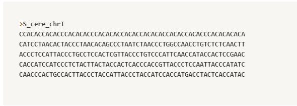
The first five lines of the FASTA for the Saccharomyces cerevisiae reference genome. The first line, starting with a greater than sign “>” contains a description of the sequence. The other lines contain the sequence.

The next step is establishing the location of the sequencing reads within the genome. To do this, the raw reads are aligned onto a reference sequence. This generates a tab-delimited text file called a Sequence Alignment Map (SAM). SAM files tend to be enormous so they occupy a lot of disk space and may take a long time to process. For easier analysis, SAM files are converted to a compressed binary format called BAM (Binary Alignment Map), which despite not being human-readable is smaller in size and easier to access using a computer.

The SAM format (Source: Samtools Documentation)

Often when studying the genetics of a population, most positions in the genomes of the individuals under study will contain the same base. Such fixed sites are not very informative and can be dropped from the analysis. Instead, we keep track of how many differences exist between the reads and the genome (i.e. “variants”), and where they occur within our reference genome. This is done using another tab-delimited text format known as the Variant Call Format (VCF), generated from mapping the reads to a reference sequence and identifying the variants.

An example VCF file viewed in a spreadsheet. VCF enables us to record variants (single nucleotide polymorphisms or SNPs, insertions, and deletions), and efficiently compress the data so that it can be indexed, accessed, and extracted quickly. (Source: EMBL-EBI Website)

Now that the data is in text format, it can be parsed and manipulated using a scripting language such as Python. 

Enter JLOH…

JLOH from the block

Developed at my host lab, JLOH identifies regions in a genome where stretches of the differences between two genomes have been lost during evolution through a process called “loss of heterozygosity”.

The sample we are using for testing is a hybrid of the yeast species Saccharomyces cerevisiae and Saccharomyces uvarum.  When used with a hybrid, the JLOH algorithm needs three inputs: 

  • Two reference sequences in FASTA format, containing the genomes of the parents of the hybrid species.
  • Two BAM files with the mapping records of the hybrid genome reads onto the two parental genomes
  • Two VCF files containing the SNPs or single base pair substitutions, representing the differences between the sequenced reads of the hybrid and the two parental genomes. 

With these files, JLOH outputs blocks of the two parental genomes where some alleles have been lost, i.e. LOH blocks.
JLOH outputs several files, the most important one being a TSV file containing the LOH blocks, aptly named jloh.LOH_blocks.tsv. These output files together with the input BAM files can be viewed in a genomic viewer and would look something like the image below and the results interpreted.

JLOH output viewed in a genomics viewer (source: JLOH GitHub)

That is it for this post. It is a long read so if you have read it all through, you deserve a pat on the back. I hope you now have a basic understanding of how a genome can be analyzed so stay tuned for the next post where I will tell you a little more about JLOH’s core functionality and what I have been doing to make sure it is fast, resource-efficient, and can scale on an HPC cluster. In case anything is unclear, please leave your question in the comment section below and we can discuss it.

Permafrost is an issue that has recently resurfaced in the global media, due to the climate change effects. In short detail, permafrost is part of the ground that continuously remains below 0 °C (32 °F) for a few years, located on land or under the ocean. Approximately 15% of the Northern Hemisphere or 11% of the global surface is underlain by permafrost, including areas like Alaska, Greenland, Canada and Siberia.

Permafrost is not necessarily the first layer above ground. It can be from an inch to several miles deep under the Earth’s surface. It frequently occurs in ground ice, but it can also be present in non-porous bedrock. Permafrost is formed from ice holding various types of soil, sand, and rock in combination.

Manifestation.

Permafrost resurfaces in large-scale land forms, such as palsas and pingos as well as smaller forms, such as patterned ground found in arctic, periglacial and alpine areas. In ice-rich permafrost areas, melting of ground ice initiates thermokarst landforms such as thermokarst lakes, thaw slumps, thermal-erosion gullies, and active layer detachments.

Contraction crack (ice wedge) polygons on Arctic sediment.

Climate change effects.

The increased heat cause by climate change has brought higher temperatures to multiple areas with permafrost, causing some permafrost to thaw. While the impacts of climate change on permafrost vary at regional and local scales, permafrost thawing has been observed in multiple parts of the world.

The thawing of permafrost however can have detrimental consequences. For example, as ice-filled permafrost thaws, it can evolve into a mud slurry that cannot support the weight of the soil and vegetation above it. Infrastructure such as roads, buildings, and pipes could also be damaged as permafrost thaws.

Our work regarding permafrost.

In our project, me and my partner @dogukant are analyzing permafrost and it’s effects with the OpenFoam solver permaFoam, while using supercompurting infrastructures.

Hello everyone. It’s been a while since my previous post since PRACE SoHPC kept me busy! Before introducing my project to you, I would like to explain some basic concepts to clarify in advance some ambiguous scientific stuff you are going to come across by following my posts. So grab your favourite snack or beverage and let me talk about some cool physics concepts!

Particle Physics Basics

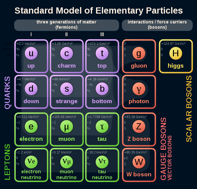
All the existent particles are divided into elementary particles and composite particles. The former ones are not comprised of other particles while the latter ones are. All charged particles are considered to have an antiparticle that has the same properties but an opposite charge. In order to classify the elementary particles based on their properties and introduce the rules of their interaction, we resolve to a theory called the Standard Model. This theory divides them into fermions and bosons depending on the particle property called spin. Fermions have a half-integer spin and obey the Pauli exclusion principle. In contrast, bosons have integer spin and don’t obey the Pauli exclusion principle.

The bosons are what we call force mediators. This means, that every particle interaction can be viewed as an exchange of a boson. The only exception is the newly discovered Higgs boson whose field is associated with giving other particles their inertial mass. Other than that, the remaining bosons are the photon, the gluon, and the W & Z bosons which are the carriers of the electromagnetic, the strong, and the weak force respectively. Moreover, each of those forces has an associated charge which particles must have in order to participate in that interaction. Therefore, there is the electric charge for the electromagnetic force, the colour charge for the strong force, and the weak charge for the weak force. An interesting fact is that, unlike electrically neutral photons, gluons and W & Z bosons carry the charge corresponding to the force they mediate. As a result, they can interact with themselves.

The fermions are the particles responsible for making up the matter and are in turn separated into quarks and leptons. Their main difference is that quarks have colour charge while leptons do not. However, both of them come up in six flavors that can be categorised into three generations, where particles in different generations have similar properties but different masses. Specifically, the existent quarks are: down, up, strange, charm, bottom, and top. The existent leptons are: electron, muon, tau, electron neutrino, muon neutrino, and tau neutrino. All those particles except for the neutrinos have an electric charge.

Basic hadron categorisation

Since we got introduced to the elementary particles, we should also make a quick reference to the composite particles. Even though they consist of hadrons, atomic nuclei, atoms, and molecules, we will be mainly interested in hadrons since the rest are a combination of hadrons and elementary particles. Hadrons are made of quarks and are divided into baryons, which have an odd number of quarks(usually three quarks), and mesons, which are made of an even number of quarks(usually one quark and one antiquark) and are relatively unstable. Due to the spin resulting from their number of quarks, baryons are fermions while mesons are bosons. The most popular baryons are protons and neutrons whereas the most popular mesons are pions and kaons.

What is Lattice Quantum Chromodynamics?

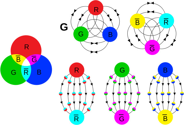
All neutral colour charge combinations

In the above section, we mentioned a new type of charge called colour charge and associated it with the strong force. Initially, we should clarify what exactly the strong force does. As we discussed, quarks are the main constituents of matter since they form the protons and neutrons, while gluons mediate the strong force just like photons mediate the electromagnetic force. However, one should wonder how quarks are bound together since their small mass could enable them to move constantly at speeds close to the speed of light. The answer to this question is that they are held together by the strong force, which is indeed the strongest of the four forces!

Now that we have understood the strong force, we need to shed some light on the colour charge. This charge has three colours red, green, blue, and three anticolours. A particle made up of all three colours or anticolours or one colour and its corresponding anticolour has a neutral colour and electric charge. The colour charge can also explain the existence of some composite particles such as the delta baryon which is constructed by the combination of three up or down quarks. Without the property of the colour charge, there would be two quarks with the same spin, which would violate the Pauli exclusion principle. Consequently, just like Quantum Electrodynamics(QED) is used to explain electromagnetic interactions, there is the theory of Quantum Chromodynamics(QCD) which describes the action of the strong force.

In physics problems, it is quite common to rely on what is referred to as perturbative solutions. This entails finding an approximate solution to a problem, by starting from the exact solution of a related, simpler problem. For instance, you can think of the Taylor series expansion of a challenging function. That would be a great way to solve QCD problems but there’s a catch. The highly nonlinear nature of the strong force and the large coupling constant at low energies makes finding perturbative solutions extremely complicated. For this reason, physicists tend to formulate QCD in discrete rather than in continuous spacetime by using a lattice. Lattice QCD(LQCD) is a non-perturbative approach that simplifies the daunting task of solving QCD problems.

What is my goal with the project?

To conclude our extensive discussion about the fascinating world of LQCD, it is about time that I describe my project’s objective. That is to efficiently use a tool called chromaform with the help of HPC resources and make several QCD simulations. The target of them is to extract successfully the mass of a pion and then find an input quark mass that would result in a pion mass close to the experimental one. Those experiments will give us a good idea of how much the input quark mass and some omitted quark-loop effects influence the resulting pion mass. In my next blog post, I will explain the whole process much more thoroughly and provide my results in its step.

Follow by Email