This project will be oriented to verify how a code related to the forecast of energy consumption is scaled from a local server to a supercomputer. This process will be implemented through Python and R in order to perform different actions required to fulfill the objective of the project.
2. Script used.
The script used has been modified in order to parallelize the code provided. Specifically, various techniques have been used, among which we can highlight the following:
Mcapply: it is one of the simplest ways to parallelize the code and, therefore, one of the most commonly used.
ParSapply: is a function that parallels the “sapply” method. This allows us to create a cluster from where the code can be executed.
ParLapply: it is a function that allows us to use the “lapply” method in parallel. In the same way, it allows us to execute the code in a cluster (previously created).
3. Comparative with server and final data.
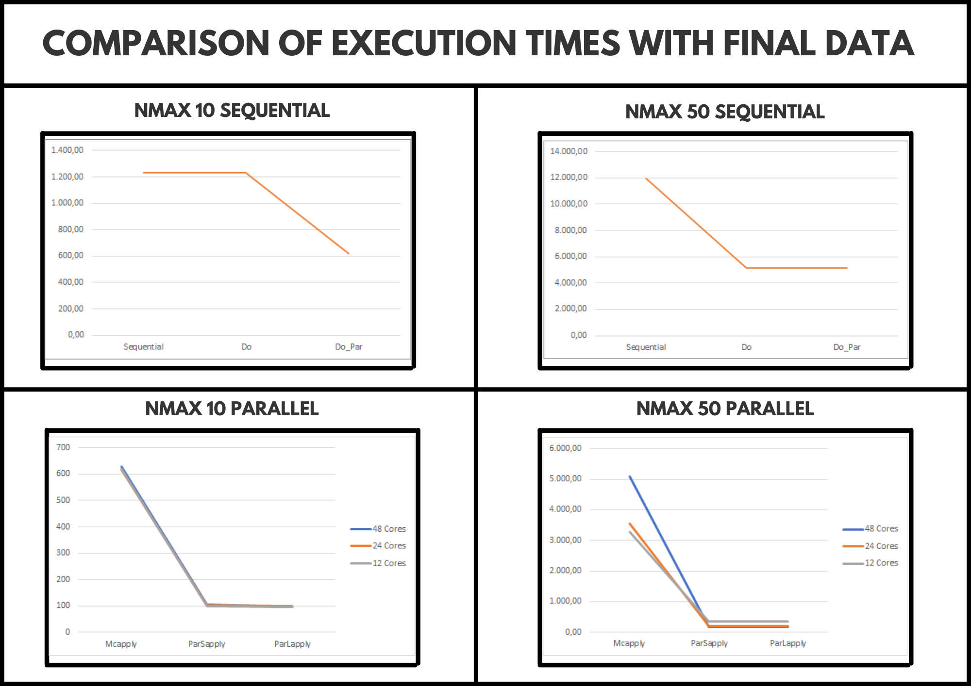
For the development of the comparison, the server provided by the research mentor has been used. By having 48 cores, the code has been executed using 48, 24 and 12 cores to obtain more complete results. It should also be noted that the code has been modified by adding a new variable called “Nmax”. This allows us to configure the size of the problem and, therefore, through logic, the smaller it is, we should obtain a shorter execution time.
After carrying out the comparison, we have detected that for a medium problem size (Nmax 10), the most optimal is to use 12 cores since they provide us with less execution time and we can leave the other 26 cores available for another execution, however, for a larger problem size (Nmax 50), we can see that using 48 cores is the most optimal option.
Finally, we can say that ParSappply obtains a shorter execution time, however, it should be noted that ParLapply has a higher time but quite similar, therefore, the most logical thing would be to use either of these two options.
These conclusions are supported under the image we can see below:
The project that we can see in this document consists of the parallelization of a code provided by the course mentor. The aforementioned code is made under the programming language called “R” and allows us to make a prediction using various statistical methods.
2. Development.
In this section, we will see how the code has been parallelized using two methods: “Doparallel” and “Lapply”. In the same way, we will see how we have modified both the sequential code and the parallel code to be able to measure the execution times of each section of interest of the code, as well as the total execution time.
2.1 Sequential time measurements.
For this section, the code provided by the mentor has been understood and has been modified following the steps that we can see below.
We have added the tictoc library.
Inside the main loop we have added the function “System.time” (it allows us to be able to measure the total execution time).
The tictoc library has been used to measure each of the parts of interest (load files, create and save the model and generate the prediction).
We save each calculated time in a separate Excel file.
2.2 DoParrallel.
For this section, we have modified the code obtained from the previous section under the following steps:
A function called “ExecuteCode” has been created that, through a parameter that we send to it, allows us to be able to carry out all the main code for a single consumer.
An external loop has been created that allows us to go through the list of consumers using a “Foreach” and the number of cores to be used has been registered.
2.3 Lapply.
For this section, the changes that we can see below have been made:
Se ha creado un clúster con 3 cores y se ha agregado a la función “parSapply” junto con el nombre de la función a ejecutar.
Se ha agregado el bucle dentro de la función para ganar mayor simplicidad en el código.
3. Comparative.
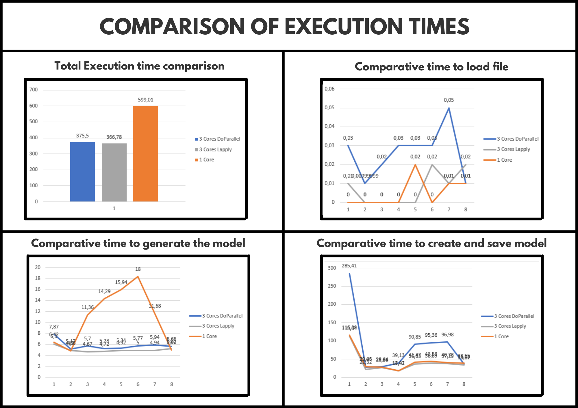
Next, we can see a comparison of the execution times obtained for each of the implementations made.
Comparison results
As we can see in the previous image, the highest execution time obtained is in the sequential version (of course). Similarly, it should be noted that the times obtained in each parallel version are more or less similar, therefore, we should not opt for any at least for now.
Hello, my name is Omar, I am 23 years old, I am a studious and enterprising boy. I did different studies in the computer area, in fact, I have a degree in computer engineering and a specialized Master in the same sector, I am currently doing the second Master in cybersecurity and data intelligence in conjunction with the PhD.
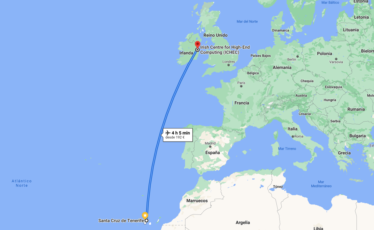
From Canarias (Spain) to the Irish Center for High End Computing
In this blog, I come to tell you about my experience in the HPC summer course, which I have had the privilege of taking from the comfort of my island, specifically, from Tenerife, in the Canary Islands (Spain), within which it is enjoyed of a totally paradisiacal climate and, which I recommend entirely. Likewise, I must emphasize that this course has been carried out through different online platforms such as, for example, the zoom platform, through which the teacher has met every day with the best disposition and encouraging us more and more, not only to internalize that knowledge but to be part of it. This experience was quite enriching, since as my university instructors previously commented to me, this opportunity allowed me to broaden my range of knowledge about the computer science area and go a little deeper into certain knowledge related to my PhD.
In my first post, I described the goals of my and Mukund’s project. We are looking to create thermal models describing the heat processes going on in regolith, the loose small pieces of rock that cover the surface of asteroids like Bennu. These heat processes are due to conduction and radiative transfers. (No atmosphere on asteroids means there is no medium for convection to occur)
My portion of the project is centered on answering the question “When a body radiates heat, where exactly does it go?”. Answering this question requires calculating the view factors of the surfaces.
Let’s consider two surfaces 1 & 2, with temperatures T1 and T2, areas A1 and A2. The rate of heat transfer from 1 to 2, derived from the Stefan Boltzmann constant is equal to R1->2 = σA1F1->2(T41 – T42). σ is the Stefan-Boltzmann constant.
That F1->2 there is the view factor from 1 to 2. Also known as the form factor or configuration factor, it describes the portion of heat that is emitted by 1 that is received by 2. My project centres on finding for each surface, as described by a triangular mesh, what other surfaces can it see, and calculating the view factor between them.
Double Area Integration
The formula defining the factor is:
for the surfaces seen here to the right. While the calculation isn’t complicated, a double area integral is going to be expensive to compute accurately when thousands of surfaces are being used. Thus other methods exist to solve this problem that I will outline
Monte Carlo Method
One alternative to the double area integral is the Monte Carlo method. Readers will likely be aware of the principle of Monte Carlo methods – that random sampling can be used to calculate numerical results, sometimes faster than deterministic methods. In this case, one can, when calculating the view factor from a particular point, dA1, choose a random angle at which to project a ray from that point, and find what surface it hits. If one repeats this process N times, and find that a surface A2 is hit x times, at N increases we know -> FdA1-> A2.
This can have the advantage that it can be done to find the factor from dA1 to multiple surfaces at the same time. However, the efficiency and convergence of this method can be variable based on the situation, and we have not chosen to use this in this project.
These are just two examples of methods that can be exercised to find the view factor. Others exist, including the Nusselt Sphere, the Crossed-Strings method and others. A good review of the matter can be found here
In my next article, I will recount my experiences implementing view factor calculations for my project
Little over halfway into the project I’ve finally gotten to grips with it. In this piece I’m going to introduce my project titled ‘Computational atomic-scale modelling of materials for fusion reactors.’
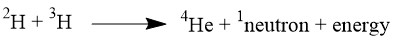
Its all comes down to energy generation. Climate change presents a growing global issue and requires a complete shift in the current energy production systems which rely on fossil fuels. Nuclear fusion was one of the ideal options to solve this problem, as it offers a way to generate carbon free power. It has been one of the ongoing international goals of science since the 1970s (Knaster et al, 2016) as a replacement for fission. The big advantage of fusion is that its major waste product is harmless helium gas. As well as this it is a controlled process without the dangerous chain reaction seen in nuclear fission. The process occurs in the sun, in which hydrogen atoms are brought together with enough force to fuse , releasing large amounts of energy (Figure 1).
Figure 1 – Simple equation for nuclear fusion using deuterium and tritium with mass numbers shown. Other fusion routes exist, for example using lithium.
A practical reactor (i.e. one which produces more energy then it consumes) has so far remained out of reach. While fusion has been performed, it is not sustainable, and as the world lacks a comparable high energy neutron source, there has been only limited work to investigate material performance under prolonged fusion (Chapman, 2021). Of course here a HPC can provide great predictive work.
Our project aims to support these efforts. The temperature and pressure conditions of such industrial reactors will be extreme and require high performance materials. Evaluation of such materials cannot currently take place as there is a lack of sufficiently high energy neutron sources (Knaster et al, 2016), limiting testing. Here computational modelling offers a way to perform these investigations in advance of real world testing, helping to speed development. Computational modelling can occur at a number of levels of scale; from ‘coarse’ representations presenting materials as continuous blocks, to full depth representations using quantum mechanical calculations to include the effects of electrons in calculations and therefore include chemical bonding. Our work takes place on the atomic level using so-called molecular dynamics. This scale allows atomic level resolution while avoiding computationally costly electronic structure calculations. It does this by representing atoms using classical physics, viewing atoms as a series of spheres which have a number of parameters controlling the forces they exert on each other, which are then calculated to give trajectories over a series of time steps. This allows large systems (Millions of atoms or micrometer scale) relevant to radiation damage to be represented.
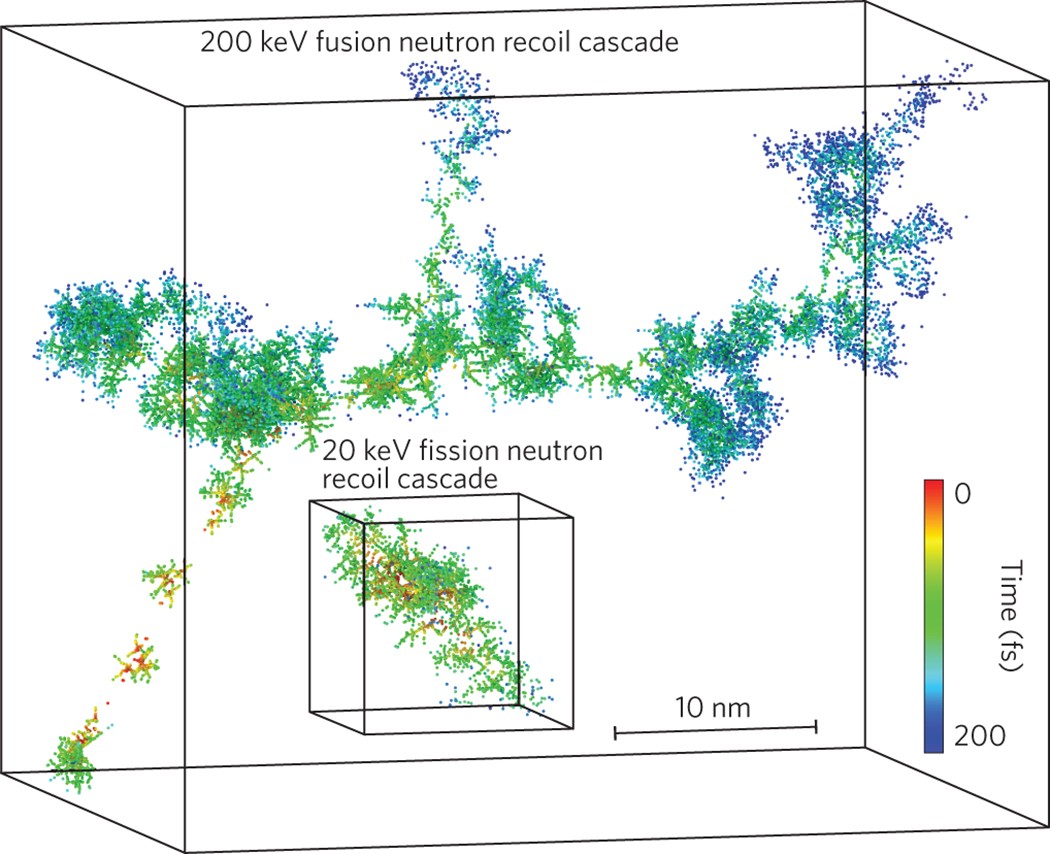
One of the favored materials for fusion reactor components is crystalline tungsten. It has the highest melting point of any element and a high resistance to sputtering (breaking apart) due to energetic particles. Molecular dynamics will allow investigation of damage cascades under neutron bombardment; the results of atoms receiving energy from oncoming neutrons and flying out of position in the crystal disrupting and mobilizing increasing numbers of adjacent atoms. This gives cascades similar to those seen in Figure 2.
Figure 2 – Evolution of two cascades in tungsten at given energies with time. Sourced from, J. Knaster, A Moeslang & T. Muroga Nature Physics, 12, 424–434 (2016)
My colleague Paolo is working on thermal conductivity measurements of such systems, and its been really interesting to see his work and perspective on things. My side of things has been to generate cascades such as those shown in the header. Its been a challenging but enjoyable project. My personal experience has been one dominated by problem solving, attempting to find out how a simulation set-up has gone wrong. Though at times this is frustrating, it is rewarding to find solutions and to expand my knowledge of the HPCs I am using. Especially as I’ve finally been able to execute defect cascades to the million atom scale.
Moving forward, Paolo and I hope to further our analysis of these reactor components and defect cascades. I will focus on comparing cascades at different energies and using various potentials (determiners of tungsten interactions), to be presented at the end of the project. This will be an opportunity to really show how our work has developed and contributes to the existing research on the massive undertaking of developing nuclear fusion. Overall, I am happy to be contributing to this area of investigation and I am hopeful for the future of nuclear fusion and how it can improve the sustainability of our world.
Bibliography
J. Knaster, A Moeslang & T. Muroga, Nature Physics, 12, 424–434 (2016)
I. Chapman, Putting the sun in a bottle: the path to delivering sustainable fusion power | The Royal Society, https://www.youtube.com/watch?v=eYbNSgUQhdY, 2021.
Hello again! It’s time for an update blog! Last time I shared some thoughts on the training week and the initial idea behind the project. Naturally, a lot has evolved since then and here I will try to explain how.
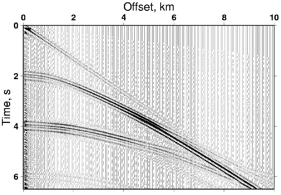
First of all, it is necessary to define the problem that we are trying to solve. And again, I will use the example from Earth Sciences. Imagine you are on land and you set up an experiment which involves using a controlled source of seismic waves (dynamite for example) and a line of receivers. The goal is to find the structure of the subsurface. You proceed with the explosion and gather wavefield data from your sensors. You use it to make cross-sections, such as the image below. The issue is that the scale is time and not distance (which we want). In order to convert it, you can think of a very simple equation: distance = velocity x time.
Seismic section. Source: Imperial College London
In order to constrain structural features (related to distance, not time), we can adopt a simple approach. We can discretise subsurface into a grid. Each box will represent one value of velocity and have defined dimensions. We take the inverse approach of trying to match the sum of distance/velocity per box over the whole path of seismic wave to the observed arrival times. This can allow us to determine what the actual structure of geological layers is.
This problem and many other similar ones can be adapted to the following form: Ax = b. This is the, so called, System of Linear Algebraic Equations (SLAE). As you can already imagine, there is a lot (!) of data involved, so any means of accelerating the computations are important. You would probably be quite disappointed if you tried to solve such problems living in pre-supercomputer era!
Moving on to our project, the approach we are using (and trying to optimise) is preconditioning. The idea is quite straightforward, we need to find a preconditioner for a given SLAE, a matrix which “simplifies” the problem when the system is multiplied by it. It can be thought of as an approximation of the inverse of matrix A. “Simplifies” means that it makes the problem more suitable for the solution methods, makes it converge faster to a solution. The hard thing about preconditioners is that there is no precise and established way of finding a good one for a particular problem. And this is where we come in. Our goal is to build an algorithm that can learn which parameter choice can lead to a good preconditioner. There is a lot it should do in a single iteration: perform random sampling or an optimisation procedure (depending on how far in the process we are), compute a preconditioner, compute a pure solution (without preconditioner) and the preconditioned solution. Over the past few weeks, we have been experimenting with different optimisation methods, including DQNs and Gaussian processes. We are yet to get our final results (which will hopefully look nice) that would be presentable. We’ll see what happens by the third and last update of this summer. Stay tuned!
Using the HPC clusters is not rocket science, but still you have to know how to do it. That’s exactly where we started before going into examining the velocity of our code and the two HPC systems ARCHER2 and Cirrus.
What code did we use to investigate its performance and to test the two HPC systems?
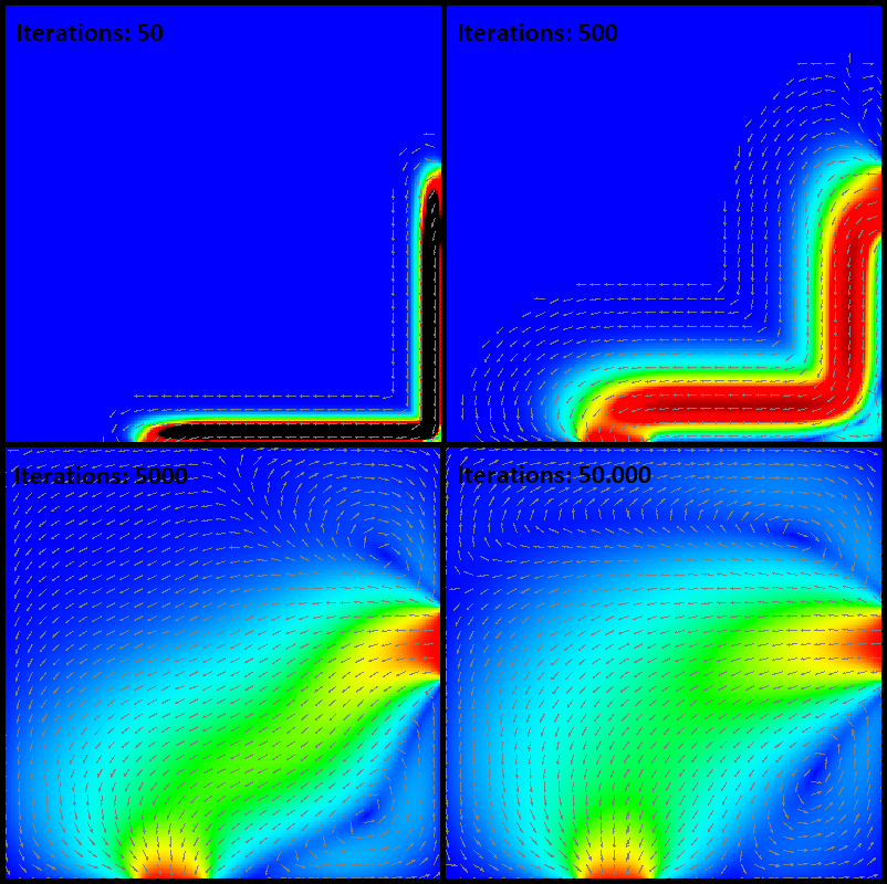
Our performance benchmark is an example from the Computational Fluid Dynamics (CFD). It simulates a fluid flow in cavity and shows the flow pattern. On a two-dimensional grid, the computer discretises partial differential equations to approximate the flow pattern. The partial differential equations, describing a steam function, are solved by using the Jacobi algorithm. It can be described as an iterative process which converges to a state with an approximated solution. Every iteration until the stable state adds precision to the results. Additionally, increasing the grid size leads to a result with higher precision but is also more computational intensive.
How does is it look like?
Approximation of the flow through a square. The flow comes from right centre and leaves at bottom centre. With an increasing number of iterations the approximation is becoming more accurate.
What language did we deal with and what did we focus on?
C, Fortran and Python. The code in C and Fortran was already there. Hence we had to translate C or Fortran into Python and make sure that they do the same. We focused on Python as it is a widely used language in science and more and more often used on HPC systems for running code. In comparison to C and Fortran as you might know, Python is slow: The readability and the dynamic typing – defining the variable type in the runtime – slows down the performance and makes Python unattractive for complex calculations with big problem sizes. At the same time, Python is popular and has a big community which means that there are solutions!
What did we use to improve the performance of Python?
Optimise: Numerical Python, named Numpy, is a specialized package which is optimized. (Surely, in the end of the project we can post some evidence!)
Divide your problem: MPI is a typical way to parallelize code. mpi4py is a package made for this purpose in Python.
Parallelize it but with much more cores: Apply your problem to GPUs
What did we measure and how?
The core of the algorithm is an iterative process. The algorithm improves with every iteration the approximation of the fluid dynamic, meaning that every iteration processes the same numeric calculation. Therefore the mean of the time of iteration provides us with information of the performance.
We coded. We tried out. We played around with alternatives. What to expect from coding on HPC Systems and what performance improve you can achieve with Python, NEXT TIME we will provide you with all the insights!
Greetings everyone. My name is Ioannis Savvidis and I come from a beautiful city named Kavala in Greece where I am writing this post. I am a Materials Science and Engineering undergraduate student at University of Ioannina with an interest in computational materials science. Growing up I had an interest in programming and its applications and I enjoyed a lot playing video games on computer with friends. For my studies I didn’t choose a related degree to follow because I had a bigger interest in chemistry, physics and engineering. That lead me to MSE department, were in my last year I chose to follow the path of computational materials science. Even though this is not a “mainstream” pathway for my department, I decided to follow it, because I see a big opportunity in advancement of new material discovery and applications.
Picture of me!
Other interests that I have are related to sports and cooking. Before the pandemic of COVID19, I used to workout a lot by going to a gym and train on Brazilian Jiu Jitsu, a ground based martial art that is focused on grappling and leverages that will lead to submissions. Other sports that I enjoy doing are snowboard in winter and sailing in summer. After the pandemic, we had to stay in home so most of my free time I would use it on cooking and watching TV series like Peaky Blinders or Better call Saul, two of the best series I have ever watched to tell the truth.
In those times a teacher associated on computational materials science suggested to me to look for SoHPC and if I am interested to any project to apply for internship. That was the first time I learned about HPC and its applications and I was intrigued and wanted to participate and learn more.
When I got the email of acceptance I was very happy that I got the opportunity to work on a supercomputer and learn a lot of new things. And so after the first training week that I found it very informative, I learned about applications on supercomputers and parallel programming. So for this summer I will be working as a team with Eduard Zsurka for Project 2108:Efficient Fock matrix construction in localized Hartree-Fock method under the guidance of Dr. Jan Simunek.
Anomaly detection is the process of accurately analyzing time-series data in real-time, identifying unexpected items or events in data sets, which differ from the norm (no anomalies). Also, it can be an extreme case of an unbalanced supervised learning problem, as the vast majority of data generated by real supercomputers is, by definition, normal. In today’s world, the issues concerning their maintenance are increasing by rapidly becoming larger and complex the High-Performance Computing (HPC) systems. Anomaly detection can help pinpoint where an error occurs, enhancing root cause analysis and quickly getting tech support before reaching a critical state.
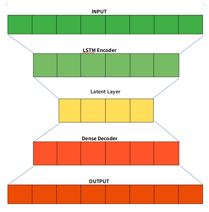
LSTM Autoencoders
Autoencoder is an unsupervised learning technique capable of efficiently compressing and encoding data and reconstructing the data from the reduced encoded representation to a representation close to the original input as possible. For using Autoencoder for anomaly detection, we first train an Autoencoder on normal data, then take a new data point and reconstruct it using the Autoencoder. If the error (reconstruction error) for the new data point is above some threshold, we label the example as an anomaly.
The bottleneck or Latent layer is the layer that contains the compressed representation of the input data. This is the lowest possible dimension of the input data.
For anomaly detection, we used an LSTM autoencoder that is capable of learning the complex dynamics of long input sequences. We used data sets that are currently being collected by ExaMon on several supercomputers atCINECA, in particular the current tier-0HPC system, Marconi100. To learn more about the data set we used, you can check my colleague’s post about it.
In my last post I had mentioned that NASA’s OSIRIS-REx, one-of-its-kind mission to collect samples from an asteroid and return to Earth, and the mission that forms the crux of my project. Personally, it is surreal to imagine such a feat being accomplished in our time. With forays such as these, space exploration surely seems to be on an exciting trajectory once again. I am writing this post to provide some context.
Asteroids offer a fascinating insight into early-universe. They are thought to contain substances from the formation of our solar system, possibly providing additional bit of information than one hopes to obtain from planets. Bennu, one of the primitive and carbon-rich asteroids, is thought to contain organic materials that could very well provide new insight into origin of life. Situated around 200 million miles away from Earth, it is classified as a Near-Earth Object (NEO). Interestingly, it is also thought to have a 1/2700 chance of colliding with Earth in 22nd Century. A combination of such factors led to it being the focus of OSIRIS-REx mission.
In our project, we focus on the material that makes up the surface of such asteroids. Assumed to be a loose, grainy material, it is thought to preserve information regarding a celestial body’s geophysical history. Chunks of such a surface could be likened to randomly packed spheres. A study of thermal properties in such a model could be related to the physical properties of the regolith, which in turn provides a better understanding of the celestial body in focus — Bennu in OSIRIS-REx mission’s case. This crux of our project is the finite element method, which is a numerical technique to solve governing differential equations of a physical model. Using this, we can predict the thermal properties such as temperature distribution, or conductivities and so on.
This mosaic of Bennu, created using observations made by NASA’s OSIRIS-REx spacecraft. Credit: NASA/Goddard/University of Arizona
Launched in 2016 by NASA’s New Frontiers program, OSIRIS-REx first reached Bennu in 2018. Initially, the probe mapped the asteroid extensively, while the team analyzed these observations to choose an appropriate site to collect samples from. The team shortlisted at least four such sites. One such sites, termed Nightingale, was earmarked to grab material (Regolith) from the asteroid. In October 2020 the probe performed a sample Touch-and-Go (TAG) event, which meant that the probe collected debris after impacting it for 5 seconds.
The TAG event consisted of a series of maneuvers, and was specified to take 4.5 hours. After descending from an altitude of 770m from Bennu’s surface, the probe fired one of its pressurized Nitrogen bottles to agitate the asteroid’s surface. The resultant dust is then collected using probe’s collector head. Once this sequence was complete, the probe fired its thrusters to reach a safe altitude again. It was expected to collect 60 grams of sample, and the extra pressurized nitrogen containers were provided in case the sample collected was insufficient. However, this isn’t the case. The sampler is thought to have impacted the asteroid too hard, leaving particles wedged around the rim of its container. The mission later reported that some of the material may have flown off into space, and that the quantity of sample collected is now unknown, as they had to abort a scheduled spin maneuver that would’ve determined the mass of collected material. The sample collected remains safely sealed now, and the probe had departed from the asteroid.
OSIRIS-REx in the clean room at Lockheed Martin in April 2016 after the completion of testing. Credit: University of Arizona/Christine Hoekenga
One of the more recent updates from the mission places the spacecraft at a distance of 528,000km from Earth. It had fired its engines on May 10 that initiated the return trip, and is expected to be on-course for a scheduled arrival on 24th September, 2023. Additionally, it had been recently revealed that the data collected by this spacecraft helped refine orbital models. Before OSIRIS-REx, scientists had expressed uncertainty owing to an unclear assessment of influence of Earth’s gravity on the asteroid. The study suggested that Bennu could make a close approach with Earth in 2135, and identified Sept. 24, 2182, as a significant date in terms of potential impact. Nevertheless, it must be stressed that there exists no apparent threat of collision.
Hi everyone! My name is Edi, I just finished my Master’s degree in condensed matter physics and I was lucky enough to get accepted to project 2108. I was born in Romania, but I did my studies in Budapest, Hungary at ELTE University. Above you can see a view of the city from the Gellért Hill. On the right, in the distance you might recognize the iconic Parliament building.
During my studies I had the opportunity to get involved in 2D materials research, I was always interested in the crossing point of physics and chemistry, where chemistry can help us design materials with specific physical properties. This can also go the other way round, when we use physics to determine the structure and properties of different molecules. The latter is the case of project 2108: Efficient Fock matrix construction in localized Hartree-Fock method. I know, I know, the name is quite intimidating, but the principle is quite simple: take a guess for the electron density of a molecule, do some simple algebra like matrix-multiplications and matrix diagonalization and in some magical way you obtain a guess for the ground state energy of the molecule.
In reality this is quite complicated due to the electron-electron interaction part of the energy: simply put it’s basically impossible to guess how multiple electrons will arrange themselves, when each of the interacts with the other. In this aspect, our situation is similar to the 3 body problem. We have to first guess the electron density of the system, and verify if it is energetically favorable, if not, we modify it and we rinse and repeat. Fortunately, we don’t have to actually understand all the steps in the algorithm ( which is an implementation of the Hartree-Fock method ) in the project, instead we are looking at how different numerical algorithms can help speed up the calculations, and how we can use the architecture of the supercomputer in Zilina, Slovakia to get the fastest results. In short, the task in not the easiest, since we must have a basic understanding of the algorithm we are modifying, but we can doing without having an in-depth knowledge of the physics. We have already come quite a long way, we managed to create a new working code, but we still have ahead all kinds of testing and optimizing steps. I plan to write about this in more detail in the next post.
And for closure, I will add a photo of myself below. I hope you are doing well with your projects, and I wait to see what we manage to achieve during SoHPC 2021. Have a nice summer!
Hello again! As I mentioned in my previous blog and week3 report, I work on a multi-label classification model on biomedical texts, during a couple of weeks I worked on how to fine-tune transformers models (https://huggingface.co/models) for required tasks.
First of all, it was really tough to train the initial model for the first time than it seems. It requires you to go dive into model architectures, understand parameters, what is going on behind the scenes, and, more importantly, implement it. I will try to explain the steps I followed and what we have achieved so far and also will try to give some institutions and resources if you are interested in more about what transformer models are.
To give a quick introduction to transformers models:
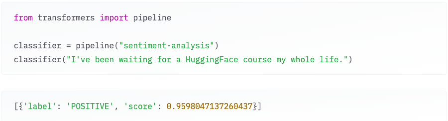
Transformer models are used to solve all kinds of NLP tasks, like the ones mentioned in the previous section. Here are some of the companies and organizations using Hugging Face and Transformer models, who also contribute back to the community by sharing their models:
Figure 1: An example of out-of-box one of the transformers models for sentiment-analysis
Step 1:
Before I talk about the first step, I want to give a brief introduction to what HuggingFace(https://huggingface.co/) is for and why we use it. As the first step, we needed to upload our dataset into the HuggingFace datasets environment (https://huggingface.co/datasets). Even if you don’t need to upload any datasets, it is sort of a convention for using HuggingFace environment like if you don’t want to spend a lot of time on uploading or dataset structure, I strongly recommend you to upload your dataset.
Our dataset includes text and label features and actually, that is all that we need to be able to train pre-trained language models for the multi-label classification tasks.
One of the inputs in the training dataset:
{"articles":[
{ "journal": "Mundo saúde (Impr.)", "title": "Determinantes sociales de la salud autorreportada: Colombia después de una década", "db": "LILACS", "id": "biblio-1000070", "decsCodes": [ "21034", "13344", "3137", "50231", "55453" ], "year": 2019, "abstractText": "El objetivo de este estudio fue analizar los determinantes sociales que afectan el estado de salud autorreportado por la población adulta colombiana. Con los datos de la Encuesta de Calidad de Vida realizada por el Departamento Administrativo Nacional de Estadísticas, DANE, en el año 2015, se estimaron modelos de respuesta cualitativa ordenada para evaluar el efecto de un conjunto de determinantes sociales sobre el estado de salud. Los resultados señalan que los factores que afectan positivamente el autorreporte de buena salud son el ingreso mensual del hogar, los incrementos en el nivel educativo, ser hombre, habitar en el área urbana y en regiones de mayor desarrollo económico y social. Los factores que incrementan a probabilidad de autorreportar regular o mala salud son el incremento en la edad, no tener educación, ser mujer, ser afrodescendiente, estar desempleado, vivir en la región pacífica y en la zona rural. Más de una década después de los primeros estudios sobre los determinantes de la salud realizados en el país, los resultados no evidencian grandes cambios. Las mujeres, los afrodescendientes y los habitantes do Pacífico Colombiano son los grupos de población que presentan mayor probabilidad de autorrelatar resultados de salud menos favorables."}
]
}
Step 2:
Before the tokenization process for the “text” feature, we need to adjust dimensions to be able to feed to the model or give the right formatted input that what the model expects. To do this we need to define how many unique labels we have among all training, validation, and test datasets. After defining this we needed to convert label feature into binary unique labels length format such as the above example that has [ “21034”, “13344”, “3137”, “50231”, “55453” ] decsCodes which also can be called class or label.
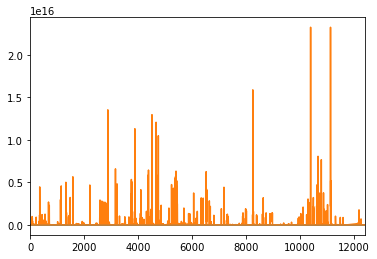
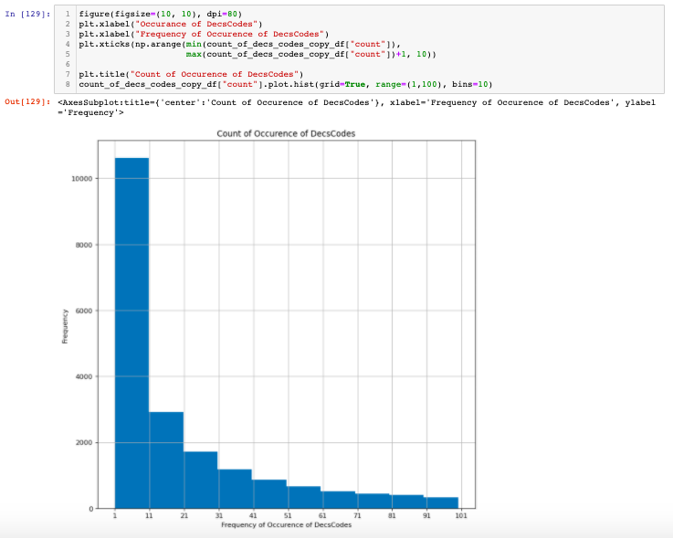
Figure 2: Frequency of DeCS Codes.
As we can see that many of the DeCS Codes have a very low count. For the scope of this problem, we could restrict ourselves to less than the amount of unique DeCS Codes. That gives us still the same 370 thousand rows of medical texts which are decent enough given that we are using pre-trained models.
The histogram plot reveals that there are almost 10 thousand unique DeCS codes that occurred in less than 10 in the entire dataset. Also in general, reducing that many unique codes still could be reasonable for the model to be able to perform classification.
After defining this we needed to convert label feature into binary unique labels length format such as the above example that has [ “21034”, “13344”, “3137”, “50231”, “55453” ] decsCodes which also can be called class or label.
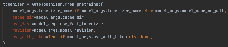
Figure 3: An Example of Tokenized “AbstractText” Input Texts Into Numerical Format that the Model Expects for Training Process
Step 3:
After some tokenization process, we need to train our model based on tokenized text and label inputs!
Step 4:
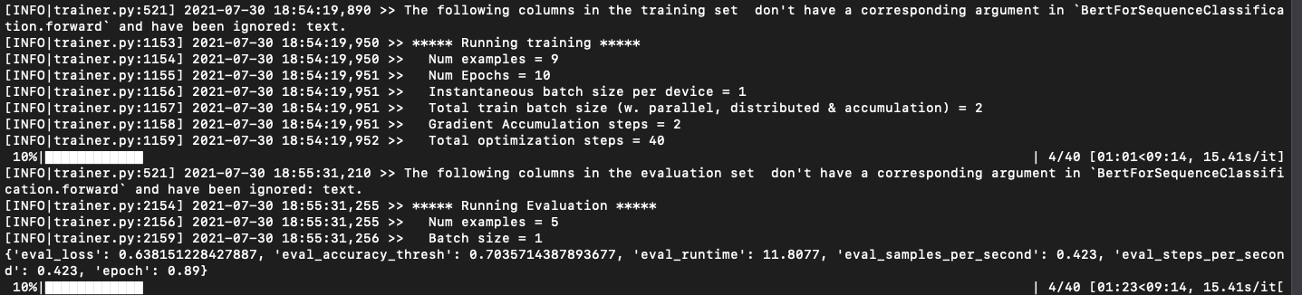
After training step, we need to evaluate our performance based on the test set that is already labeled and maybe change some hyperparemeters and tweak the model for better accuracy,
Model Name
Epoch
Accuracy
mBERT
1
0.873
BETO
1
0.8723
BioRoBERTa
1
0.8704
Table 1: Accuracy Results Table for Epoch 1
Model Name
Epoch
Accuracy
mBERT
4
0.8596
BETO
4
0.8613
BioRoBERTa
4
0.8716
Table 2: Accuracy Results Table for Epoch 4
According to the final results, each model have very close accuracy to each other. Increasing epoch from 1 to 4 does not improve accuracy much as the models might have started to overfit the training dataset more thus accuracy might be started to reduce at some point. To overcome this obstacle, EarlyStoppingCall- back class from the Huggingface library can be used for future improvements to be able to prevent and stop learning once models might reduce the accuracy. If you have any questions I am more than happy to answer! You can find a more detailed explanation on my final report, thank you for your attention! 🙂
This was such an entertaining and informative summer for me, I would like to thank my mentors for making this program very insightful! I strongly recommend the Summer of HPC program to people who are interested in HPC!
Hi everyone! I hope all you are being-well. Before I tell my SoHPC adventure with you, I would like to briefly inform you about our project which is called “Re-engineering and optimizing software for the discovery of gene sets related to disease”. Analysing and interpreting biological data in a computer environment have been made it possible by help of the developing technologies. This technology is used in kinds of different and wide areas, from network and system biology to drug researchs. In this project the affect of genetic factors with pathway analysis on the disease susceptibility on the genetic basis level has been investigated. The motivation bedin the project is optimizing the Genomicper package, which was written was previously written in R programming language, to enable it to work with larger data sets. Because as the data size increases, the number of genes that can be examined and therefore the diseases that can be detected also increases. Besides, resent technologies provides an opportinity to work with larger data sets.
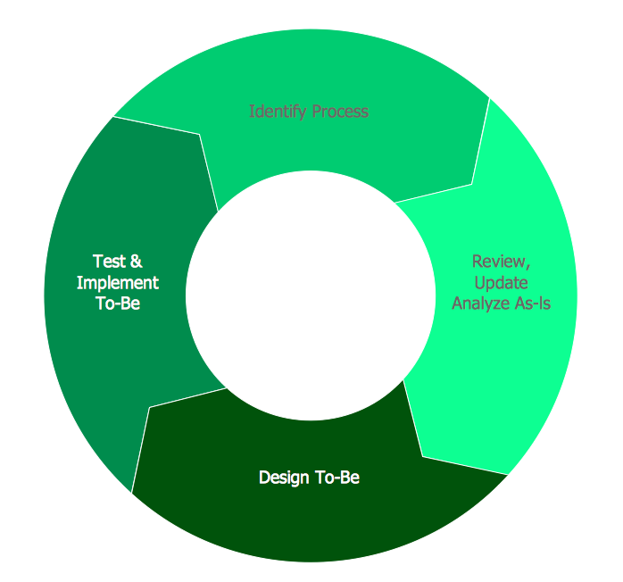
The Genomicper Package Optimisation
Figure 1: Flowchart of the project
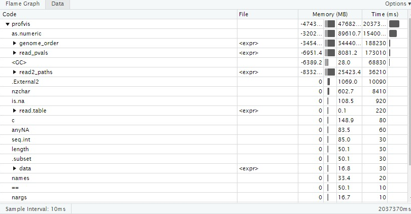
Optimization process starsts by profiling the code to detect most expensive routine in the Genomicper package according to the process time and memory usage. Then the code is optimized by algorithmic or with aim of making package use less memory if possible and to run faster. After these change, the outputs of the code will be checkedto be correct. The rewritten code is tested with different sizes of the data sets to detect the next block to be optimized.
Figure 2: An example of the profiling the Genomicper Package
Future Plan Optimization process above will be done to until no more meaningful improvements can be made to the code. Then the Genomicper package will be parallized in R language.
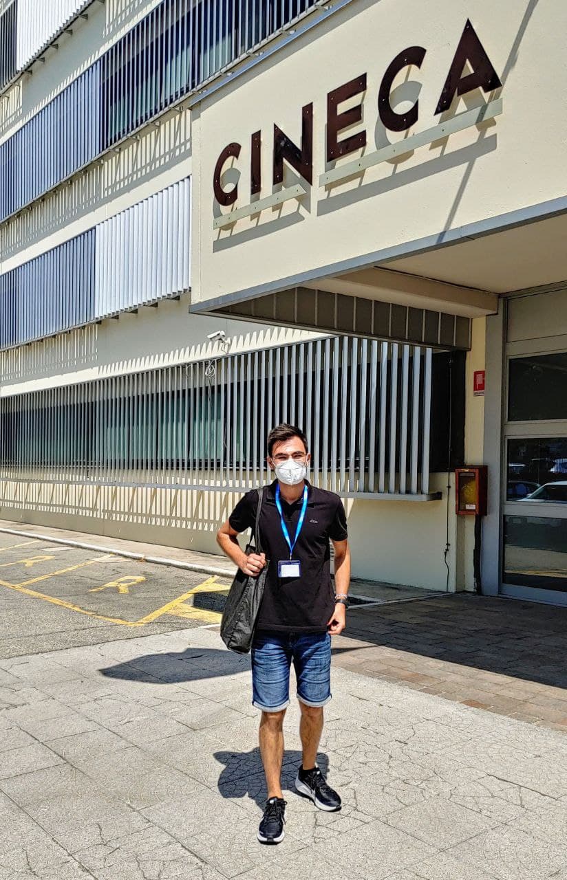
In a normal summer, all of the Summer of HPC (SoHPC) interns would stay at one of the PRACE’s 26 national supercomputing member institutions. As, of course, this is not a normal summer, the SoHPC 2021 has been designed as remote program in this year. This means unfortunately, that experiencing the everyday life at a HPC institution, and working with like-minded HPC practitioners on site is not possible. However, on the upside, remote working also grants a large degree of freedom for both work and life. This is why I decided to think positively, seize the opportunity, and set out on a journey with my laptop, which led me to the PRACE site that is associated with my project: CINECA in Italy!
My visit to my supervisor Massimiliano Guarrasi at the CINECA headquarters in Casaleccio di Reno, Bologna, Italy.
CINECA is a non-profit consortium comprising of more than 70 Italian universities and research institutions, and is located in Casalecchio di Reno, a small town close to Bologna.
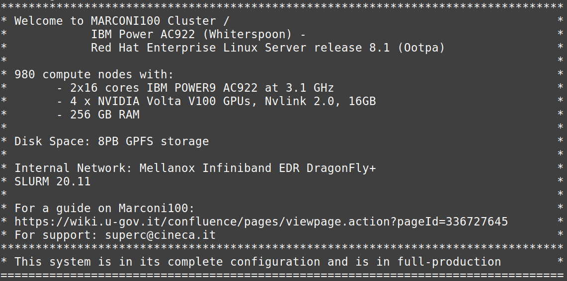
There, I was welcomed by my CINECA supervisor, the HPC specialist Massimiliano Guarrasi. Once I obtained my visitor badge, we opened the “chamber of (HPC) secrets” and entered the machine room with a specialized guide. Setting foot in this room is exciting, but also dangerous. In case of an emergency, such as a fire, it is flooded with argon within only ten seconds. The warmth and noise inside the machine room was overwhelming and made me aware of the power of the supercomputers that we are working with. One of them is MARCONI100 (M100), named after the Italian radio pioneer Guglielmo Marconi.
How powerful is our supercomputer?
To get an idea of how powerful M100 is, I would like to show you some numbers. While a conventional desktop computer possesses 4 cores (computing units), M100 features a whopping 31360 cores, that is about 8000 times as many!
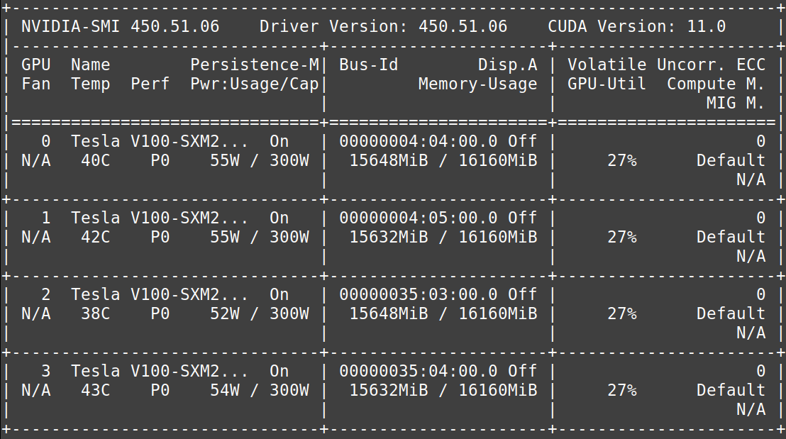
Importantly, M100 is a so-called accelerated system. That means it does not only rely on central processing units (CPUs), but also graphical processing units (GPUs). In an everyday context, you know GPUs for making possible video gaming with excellent, high-resolution graphics. In research and industry however, GPUs are utilized to execute certain parts of a program in parallel, which is typically much faster compared to conventional CPU computing. This means a significant advantage for applications such as molecular simulations, image processing, or deep learning. Using GPUs for these applications is also known as general purpose computation on GPUs (GPGPU). For GPUs by the company NVIDIA, this is frequently done using a programming technique known as CUDA.
Logging into the MARCONI100 supercomputer.
On the M100 supercomputer, we have access to NVIDIA Volta V100 accelerators, which have been claimed to train a neural network up to 32 times faster compared to a CPU! Together with the Tensorflow framework for GPUs that we are using to tackle our submarine classification problem, we can train our deep learning models much faster. Each node of the M100 supercomputer features four V100 GPUs, which me and Raska are using to train our artificial intelligence models in parallel. While I thought this to be quite complicated, using CUDA turned out to be not that difficult, and I soon started to love using the power of accelerated computing!
Accelerated training of a neural network using four NVIDIA Volta V100 GPUs.
The race towards exascale computing
Similar to the moon race, there is also a prestigious race in supercomputing: the goal is to build the first exascale supercomputer. Exascale refers to the number of calculations per second (floating point operations per second, FLOPS) that a machine is able to perform, which is a truly gigantic number: 1 exaFLOPS per second means 1018 (1,000,000,000,000,000,000) operations per second, a number that is about as large as the (estimated) number of sand grains on earth. Computing on this scale would enable us to achieve even better predictions, for example regarding the discovery of novel materials. Even large-scale brain simulations could be feasible! CINECA is one of the institutions leading the race towards this new era with its pre-exascale Leonardo supercomputer, which is part of the European Joint Undertaking EuroHPC.
You might ask yourself how supercomputing and exascale computing impacts your life. This CINECA video holds the answer:
To sum up, working with GPU-accelerated high performance computing systems is both powerful and exciting. In the future, the number of accelerated supercomputers is likely to grow.
I am curious to learn about your experiences: have you ever utilized GPUs for your computations? Do you have an application, where you think an accelerated supercomputer could be useful? Do you have experiences with remote working? Please let me know in the comments!
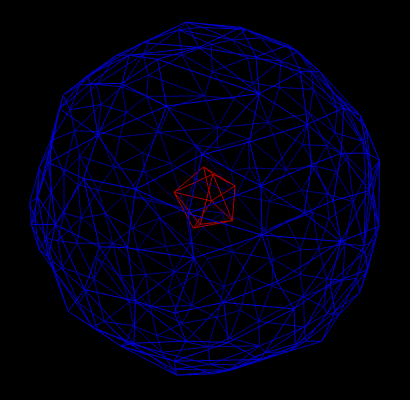
Last year, a first program has already been implemented. This program computes a triangulation that approximates the surface of a molecule. This year we are focusing on improving efficiency and adding new features. One of these new features I will present to you now:
Figure 1: The surface is a composition of an inner surface (red) and an outer surface (blue).
It may happen that the result of the computation yields several disconnected surfaces (see figure 1). However, in applications, one is often only interested in the outer surface. If we look at the picture, it is easy for us humans, to say which triangle on the triangulation belongs to which surface. However, for a computer, it isn’t as easy as it might seem at first sight. For applications, it is important to distinguish different connected surfaces automatically. Therefore, we need an algorithm to tackle this problem (and this algorithm should be ideally efficient).
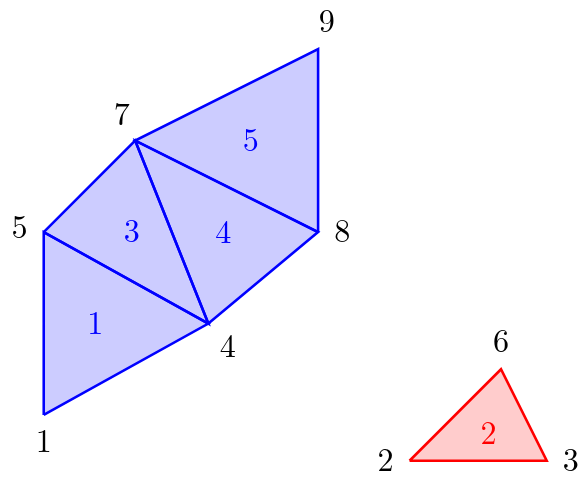
For the computer, the computed triangulation of the program is just a bunch of triangles. An example, how a triangulation looks like, is depicted in figure 2. The computer has knowledge of local connectivity in the sense that the vertices of a single triangle are connected to each other and must therefore lie on the same surface. But if we look at two arbitrarily chosen vertices of the triangulation (for example vertex 1 and vertex 9 in figure 2) it is not apparent if these two vertices lie on the same surface or not, by looking only at the list of triangles and vertices which are stored in memory. But can the computer combine the local knowledge to obtain global information about the surfaces? And if so, how is this done most efficiently?
Triangulation stored in Computer
Visualised Triangulation
Figure 2: Example of a triangulation
One solution to this problem is to use the Disjoint-set data structure (also know as Union-find data structure or merge-find set, for more details see https://en.wikipedia.org/wiki/Disjoint-set_data_structure). This data structure stores a collection of non-overlapping sets. In our case, each set consists of all vertices of one connected surface. If we look again to figure 2, we would have the sets {1, 4, 5, 7, 8, 9} and {2, 3, 6}.
In our program, the disjoint-set structure is implemented with a so-called “disjoint-set forest”. A forest is a set of trees (see figure 3). In our algorithm, we start with an “empty” forest (i.e. we have no trees at all). By going through the list of triangles sequentially, the trees are constructed little by little. If you are interested in more details I can recommend reading https://www.geeksforgeeks.org/disjoint-set-data-structures/ and http://cs.haifa.ac.il/~gordon/voxel-sweep.pdf. In our example from figure 2, the resulting forest consists of two trees. Each tree contains the vertices of one surface. As soon as we have constructed those trees, distinguishing different surfaces is relatively easy. If we look at a vertex on the surface, we can traverse up the corresponding tree up to the root vertex. If two vertices lie on the same surface, the corresponding root vertices match. Conversely, if the vertices do not lie on the same surface, the corresponding root vertices are different.
Figure 3: Example of a forest consisting of two trees.
I hope you enjoyed reading this blog post. Describing all the details of how the algorithms works would blow up the length of this post, but if you are interested in further details you are welcome to ask questions in the comments section.
The reasons why my colleague and I have decided to choose project 2109 ‘Benchmarking HEP workloads on HPC facilities’ are several. Unravelling the deeper reasons behind the project, we find a very interesting collaboration that emerged in 2020 between CERN, PRACE and other organisations with the aim of joining forces to improve the HPC world. That is why, in this post, we will describe in more detail where this collaboration comes from and what are its objectives in case it could be of interest to readers.
As is common knowledge in the world of supercomputers, as science advances the technological resources needed to sustain the necessary computing power are increasing. This is why, in order to make the most of the different existing heterogeneous architectures, a collaboration has arisen between different pioneering entities in high-performance computing (HPC). The members of the collaboration are CERN, the European Organization for Nuclear Research; SKAO, the organisation leading the development of the Square Kilometre Array radio-telescope; GÉANT, the pan-European network and services provider for research and education; and PRACE, the Partnership for Advanced Computing in Europe.
This is why this collaboration arises from the need to join forces in order to obtain better results from HPC calculations. This is where the project that my colleague and I are carrying out comes from. During the first 18 months since the agreement was signed between the different partners, the objective has been to develop a benchmarking test suite and a series of common pilot ‘demonstrator’ systems.
The purpose of developing this Benchmark Suite is to determine the different performances that supercomputers within the reach of the four participating entities can have for the development of high-energy physics and astronomy calculations. Regarding the project related to the SoHPC that my colleague Miguel and I are carrying out, we are currently trying to implement the Unified European Application Benchmark Suite (UEABS) used by PRACE in the Benchmark Suite developed by CERN. UEABS is a set of currently 13 application codes taken from the pre-existing PRACE and DEISA application benchmark suites, and extended with the PRACE Accelerator Benchmark Suite.
Not only that, but one of the main aims of this collaboration is the development of training programmes so that researchers will be able to make the most of the different existing HPC architectures. So the roots of this project lie not only in scientific study, but also in the possible training of people so that science can continue to advance.
My colleague and I are very proud and excited to be able to contribute to a project that is the result of a collaboration between four pioneering European organisations with computational resources available all over the world. That is why, with this post, we encourage you to find out more about it through the news published on 20 July 2020 on the official CERN website, whose link you can find here.
See you soon in the following post!
María Menéndez Herrero, Miguel de Oliveira Guerreiro
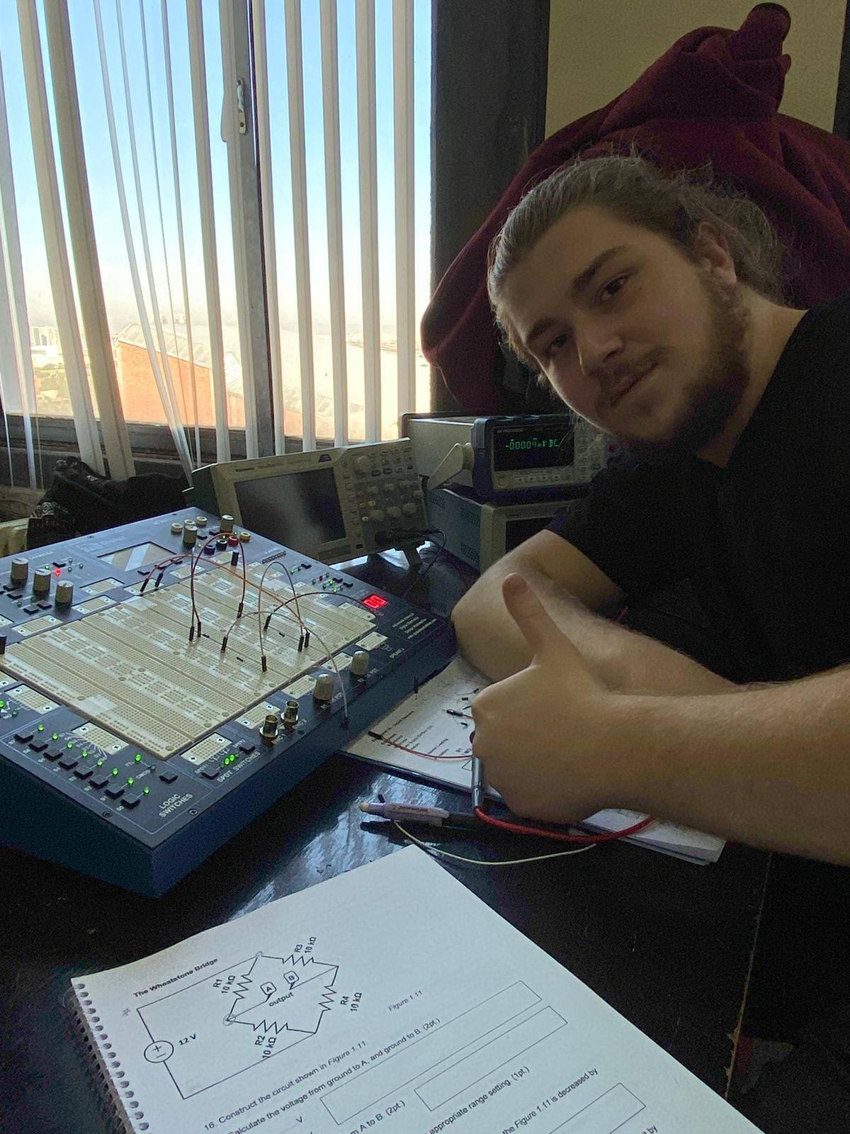
Hello all! My name is Bartu. I am an aspiring senior physics student at Middle East Technical University, Turkey. I have previously worked on large scale Arduino based data acquisition systems in an experimental physics laboratory. With the pandemic, I shifted to computational physics and since then I have been developing a molecular dynamics software with another colleague. I am also occasionally attending the QBronze quantum computing workshops as a mentor organized by QTurkey and developing a convolutional neural network for mineral composition prediction at METU ROVER.
I also play rhythm and bass guitar in a local metal band and I am interested in Brazilian jiu-jitsu. Which were all sadly postponed due to the pandemic. I would love to chat with anyone having similar interests!
This is me tired after an electronics lab session.
I am working on the “S-gear geometry generation and optimisation algorithm based on transient finite element mechanical/contact analyses” project at University Of Ljubljana. Even though I am a physics student, working on a project from a different discipline is really exciting for me. I will be posting more about the project as well so stay tuned if you are interested!
I would also like to thank PRACE and the SoHPC coordinators for organizing this amazing program allowing us to work with experts from different countries! I hope this summer will be a great learning experience for all of us! See you all later in other blog posts!
Hello again! I am halfway through my Summer of HPC adventure and would want to update you on what I’ve been doing during last few weeks. If you read my introductory post (if you didn’t, I encourage you to do so), you already know I am working on project focused on deploying machine learning applications on edge devices.
What are edge devices?
There are multiple different (but similar) definitions of the edge devices but the one I am using is that this is device which is physically located close to the end user, so it can be laptop, tablet, smartphone, single-board computer like Arduino or even simple sensor like hygrometer which is capable of saving and sending measured data. In our project, we aim to deploy machine learning application on an average smartphone.
What are deep neural networks?
Machine learning model we chose to deploy is a deep neural network (DNN). Neural network is a model which is loosely inspired by human brain. It consists of multiple layers of nodes (called neurons) which are connected with each other. Adjective “deep” means that network consists of multiple layers (usually five or even more). Each neuron in each layer has weights, which are trainable parameters representing the knowledge that neuron gained from data during training process. Picture above represents simplified schema of shallow neural network. Schema of DNN wouldn’t be much different, it would just have more layers in hidden layer(s) part.
Deep neural networks are nowadays the most popular and usually the best performing machine learning models. They aren’t ideal though. Some of the cons of neural networks are lack of interpretability, very long training time, long inference time and very often huge size of files containing pre-trained network. Latter two cons are the biggest problems when it comes to deploying neural networks on edge devices.
Why do we want to deploy machine learning apps on edge devices?
Theoretically, we could leave pre-trained models on HPC clusters or cloud servers but practically it’s often not a good choice. For example, if we want to pass sensitive data to the model deployed in cloud, we would have to send it through the internet what always causes security concerns and risk of sensitive data leak. Moreover, storing the model on edge device allows to use it even when we don’t have internet connection available. Even if internet connection is available, local inference avoids latency, which is inherent part of communicating with server through the internet.
So, what can we do to deploy DNN on the edge?
There are multiple techniques allowing to compress and optimize DNNs for the inference process. While during first three weeks I was focusing on the basics of training the DNNs and introduction to GPU and distributed training, lately I was trying and investigating one of the most popular ways to both compress the model, and make the inference faster – pruning. In its simplest form, model pruning sets specified fraction of DNN weights with smallest absolute value to 0. This makes perfect sense, as when we pass the data into the DNN, data is multiplied by neuron weights to get the output. Obviously, multiplying number by value (weight) almost equal to 0 yields result which is almost equal to 0, so by setting such a weights to 0, we are not losing much information and we don’t change our model too much. On the other hand, model which contains a lot of zeros is easier to compress and its inference process can be optimized – many multiplications by 0 are fast to perform as their result is always 0. Picture below shows the idea of pruning by visualization of model presented on picture above after pruning which set to 0 roughly 50% of neurons’ weights.
Below, you can see some charts from conducted experiments with pruning. First of all, I have to mention that I experimented with shallow model (less than 10 layers) and small dataset, as I couldn’t afford learning deep model on proper data as it would take a lot more time, and I wouldn’t manage to do much besides it. That’s why training of a single model took only around 11 minutes and unpruned model had size of around 10 MB. Plots below visualize change of compressed model size, model accuracy and training time with change of final model sparsity – final sparsity is the fraction of model weights set to 0, e.g. sparsity 0.75 means that 75% of the weights were set to 0.
I think that’s everything I wanted to write in this post! It became pretty long anyway (I tried to be as concise as possible but as you see a lot is happening), so I hope you didn’t get bored reading it and you reached this point. If you did, thank you for your time and stay tuned, as in upcoming weeks I will train deep model on big dataset using Power9 cluster and experiment with other methods of model compression & optimization!
Hi all! In my first blog post, I briefly described the project. In this post, I will mention more about the strategy of the project. More information about project 2114 is here.
Current technology developments enable us to analyze more than 30 million genetic data points to determine their role in disease. This project will focus on re-engineering genomicper which is an R package, currently available from the CRAN repository, written before. Due to this, it can swiftly analyze larger and existing data sets.
What’s genomic permutation?
Genomic permutation, shortly Genomicper, is an approach that uses genome-wide association studies (GWAS) results to establish the significance of pathway/gene-set associations whilst accounting genomic structure. The goal of genome-wide association studies (GWAS) is to find single nucleotide polymorphisms (SNPs) that are linked to trait variation.
Project 2114 aims to re-engineer the genomicper package so it can analyse bigger and existing data sets quickly. The learning outcome of this project is to learn and implement the process of optimising a real-life piece of code.
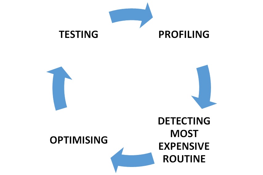
Project Life Cycle
The general strategy cycle of the project: profile the code using data sets to determine the computational and memory expensive routines. Potentially there are 8 routines to be improved. From this profile, pick the most expensive routine to improve the efficiency, iteratively optimise the routine using microbenchmark and other optimisation techniques. More information about microbenchmark here. Test the code and compare the results produced with the original routine. Continue this cycle until code performance cannot be improved any further at which point other possible improvements will be noted, e.g. rewriting code in C, parallelisation strategies, etc. Proceed to the next routine. Once all routines have been optimised look at the strategies for further improving the code.
So Far, So Good
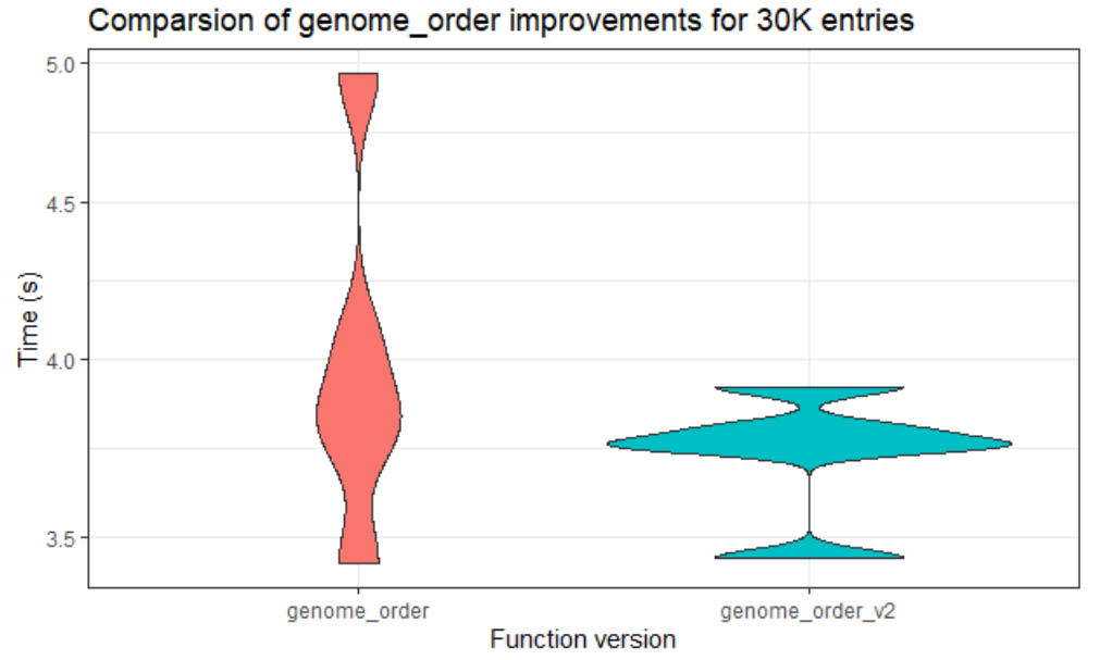
Thanks to the support from our mentors, we have made good progress. Until this week, the team managed to work with the lower data sets. We tried to analyze the existing performance, then optimized routines. The team tried to make the code more efficient also faster in larger data sets. While doing this, they used some of the fastest among R’s special functions. Through the analysis of the code, we attempted to make changes around the code. You can see one of our comparison results of the original code and the other version that we did in the below figure.
Comparison of the original routine and the optimized version 2 routine.
“genome_order” is the most expensive routine. We can clearly see that version 2 is faster than the original code. This helped very, especially since we made the most expensive routine efficient.
Upcoming weeks
In the upcoming weeks, all 8 routines will be optimised. After that, consider further performance improvement techniques. Once we have done all, we will try to improve the parallelisation of the code. I believe that the project process will continue well in the remaining weeks!
That is all for now. If you have any questions, I will be happy to answer.
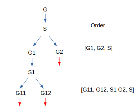
Hi ! I hope you’re ready to dive with me into this specific algorithm which will provide us a solution to our last problem. If you remember correctly, our goal is to find an order for all the nodes in a graph so that, by executing elimination, we can compute an approximation of its tree-width (max degree of nodes eliminated, we want that max as low as possible). To find this order, one well-known approach is the nested dissection. Nested dissection consists in taking a graph, computing a separator (a set of nodes), with which you cut the graph in 2 parts (or more) i.e 2 disjointed sub graphs. Repeat the same process on the 2 sub graphs until they verify some properties like “is a tree” or “is complete” where it’s easy to compute their order and tree-width. To create the final order for the root graph, start from the end by adding separators then graph orders (when they verify the previous properties and are computed directly). For instance let’s say you had a graph G, its separator is S and it splits G in G1 and G2, at this point the order is [order(G1), order(G2), S] (I write S but in reality we append all of its nodes and order doesn’t matter inside S, the only important thing is that S is after G1 and G2) . Now let us start to nest things with G1 and suppose that G2 can’t continue because it is complete. G1 will be split using S1 and its sub graphs are G11 and G12. At this point the order is the following: [order(G11),order(G12), S1,order(G2), S]. For the sake of simplicity, we will suppose that G11 and G12 are also complete to end the example here. Just one note here, our order [order(G11),order(G12), S1,order(G2), S] and this one [order(G11),order(G12),order(G2), S1 S] lead to the same tree-width so picking one or another depends on your choice when thinking about implementation. Another way to think about this approach is more visual and involve a tree like this. Therefore, the choice depends on how you want to iterate through this graph.
Nested dissection a tree (order of subgraphs is a choice between DFS or BFS)
With that in mind we can keep going on, one question you might have is “that’s nice and all, but how do you choose your separator S at each step?” The answer is the main part of the algorithm developed by Michael Hamann and Ben Strasser in this paper. Their idea is to find a balanced a cut which splits the graph in 2 balanced parts. A cut is a set of edges (usually on directed graphs are used, so it would be arcs not edges, but in our case we consider only non directed graphs) each of those edges is a pair of nodes (u,v) so that u and v are not in 2 different sets V1 and V2 which partition all nodes V (all the vertices/nodes) = V1 U V2. To get a separator from a cut we just choose randomly 1 node per edge in the cut.
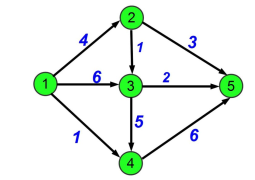
Now, onto the main part: how to select a good cut ? One specific idea in graph theory will help : the notion of flow. In some engineering problems, like computer networks, or transporting water through several pipes, you want to use the network at its maximum capacity to transport the largest amount of information or water depending on the problem. A flow is an integer value between 0 and C where C is the capacity of the pipe (i.e the maximum amount of water/info/whatever you can put in it). We also introduce 2 notions for nodes, source and target. Basically a source node is a node which creates flows so it can throw more than it receives. The opposite is the target node which absorbs flows so it can receive more than it gives. The other nodes respect the flow conservation i.e same amount of flow in and out. Here is an example of a flow graph with 1 as the source and 5 as a target, the current flow is 11 (=4 + 6 +1) and in other nodes we can see the conservation law for instance in node 2 we have 4 in and 3 + 1 out.
Example of flow graph
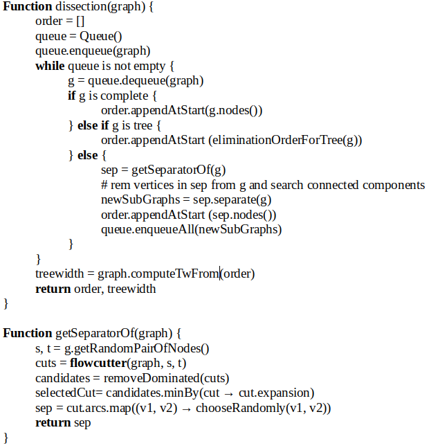
Finding the best way to flood a network to transport things from a source node to a target node is a well-known problem and it is demonstrated that finding the maximum flow is equivalent to find a minimal capacity cut. This is one of the core ideas behind the algorithm which I will explain. Another key idea is that we want a “balanced” cut which means a cut with minor difference between sizes of the 2 split vertices sets. They introduce a parameter to count this, epsilon = 2 * max(|V1|, |V2|) / n – 1 called the imbalance rate, in the core dissection part they precise to reject a cut with imbalance > 60%. To select a cut from the output cuts of the flow-cutter algorithm we will first remove the “dominated” ones i.e the ones having bigger size and bigger imbalance rate than any other one. Once we remove the worst cuts we choose the one with min expansion = size / min(|V1|, |V2|). Those wrapper algorithms can be described more easily as a pseudo code (syntax is kind of my custom fusion between Kotlin and Python) like this one :
Pseudo code of the nested dissection and separator algorithm wrappers of flowcutter
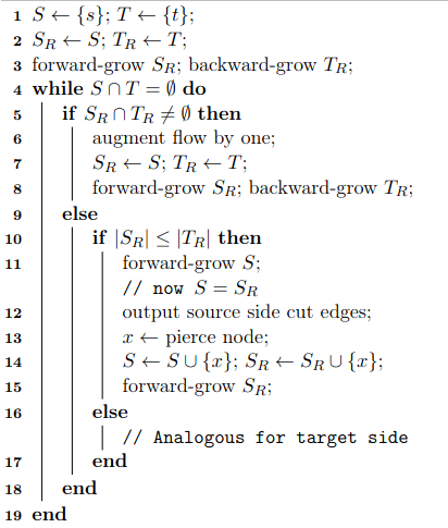
Now it’s time to explore how the flow-cutter algorithm works and how it chooses cuts. We will use the idea of flows on undirected graphs so we double each edge to 2 arcs in both directions. All the capacities will be 1 because we don’t have capacities in the input graph we use and also because it has a clever simplification with residual graphs that we no more need to compute. The algorithm will manage 4 sets of nodes S, T, SR and TR which mean sources, target, source-reachable and target-reachable. The idea is to solve the max flow problem, find the min cut and then add source (if source reachable size is too small) or target (if target reachable size is too small) in order to enhance the cut’s balance by resolving the max flow problem and repeating the process several times to get more and more balanced cuts. The pseudo code given in the paper is the following :
Pseudo code of the flowcutter algorithm
Here, the forward and backward grows are equivalents to the same process : add to the input set all the nodes such as a non-saturated path, between x in input set and y not in input set, exists. Parenthesis : forward and backward are the same because we work with undirected graphs, the difference is the direction x -> y (forward) or y -> x (backward) if you work with directed graphs. The line 12 means create cut and add it to the cuts to return at the end of the algorithm.
In a future article we will talk about complexity and performance of this algorithm on real graphs; Also will see more practical implications to enhance its result and runtime using some multi-threading.