[Video] Hi from Dublin everybody! Welcome back to my blog or welcome for newcomers.

If you have missed it, my previous blog post is available here! No worries, there is no need to read it before this one to understand today’s topic. You can read it after to know more about me if you want, but follow and stay tuned until the end of this post because I have a special announcement for you to do!

Before explaining how you can make your computer run your applications faster, I just wanted to come back quickly to our training week in Bologna, Italy, and make a point with you on my current situation.

Training week summary

As a picture is worth a thousand words, I let you discover by images the summary of this amazing training week.

SoHPC 2019 training week summary by images

Where am I now?

Since the 6th of July, I am in Dublin with Igor, another PRACE SoHPC 2019 student. We are both working on our projects at ICHEC (Irish Centre for High-End Computing), an HPC Center. Paddy Ó Conbhuí (my super project mentor at ICHEC) and I are dealing with a parallel sorting algorithm: the parallel Radix Sort, which is my project.

Enough digressions, you are most probably here to read about application and computer speed.

Pursuit of speedup

To make our applications and programs run faster, we have to find first where, in our programs, computers spend most of the execution time. Then we have to understand why and finally, we can figure out a solution to improve that. This is how HPC works.

  1. Identify the most time-consuming part of a program
  2. Understand why it is
  3. Fix it / Optimize it
  4. Iterate this process again with the new solution until to be satisfied with the performance

Let’s apply this concept to a real-world example: how can we find a way to improve programs in general? Not a specific algorithm or program but most of them in a general way? It is an open and very general question with a couple of possible answers, but we will focus on one way: optimize sorting algorithms. We are going to see why.

How do computers spend their time?

We have to start by asking what takes time and can be improved in computer applications. Everything starts with an observation:

“Computer manufacturers of the 1960’s estimated that more than 25 percent of the running time of their computers was spent on sorting, when all their customers were taken into account. In fact, there were many installations in which the task of sorting was responsible for more than half of the computing time.”

From Donald E. Knuth’s book Sorting and Searching

In 2011, John D. Cook, PhD added:

“Computing has changed since the 1960’s, but not so much that sorting has gone from being extraordinarily important to unimportant.”

From John D. Cook, PhD in 2011

Why this still might be true nowadays?

It is become rare to work with data without having to sort them in any way. On top of that, we are now in the era of Big Data which means we collect and deal with more and more data from daily life. More and more data to sort. Plus, sorting algorithms are useful to plenty more complex algorithms like searching algorithms. On websites or software, we always sort products or data by either date or price or weight or whatever. It is a super frequent operation. Thus, it is probably still true that your computer spends more than a quarter of its using time to sort numbers and data. If you are a computer scientist, just think about it, how often did you have to deal with sorting algorithms. Either wrote one or used one or used libraries which use sorting algorithms behind the scene. Now the next question is what kind of improvement can be done regarding sorting algorithms? This is where the Radix Sort and my project come into play.

Presentation of the Radix Sort

It has been proved that for a comparison based sort, (where nothing is assumed about the data to sort except that they can be compared two by two), the complexity lower bound is O( N log(N) ). This means that you can’t write a sorting algorithm which both compares the data to sort them and has a complexity better than O( N log(N) ). You can find the proof here.

The Radix Sort is a non-comparison based sorting algorithm that can runs in O(N). This maybe sounds strange because we often compare numbers two by two to sort them, but Radix Sort allows us to sort without comparing the data to sort.

You are probably wondering how and why Radix Sort can help us to improve computer sorting from a time-consuming point of view. We will see it after explaining how does it work and go through some examples.

How does Radix Sort work?

Radix sort takes in a list of N integers which are in base b (the radix) and such that each number has d digits. For example, three digits are needed to represent decimal 255 in base 10. The same number needs two digits to be represented in base 16 (FF) and 8 in base 2 (1111 1111). If you are not familiar with numbers bases, find more information here.

Radix Sort algorithm:
Input: A (an array of numbers to sort)
Output: A sorted

1. for each digit i where i varies from least significant digit to the most significant digit:

2.     use Counting Sort or Bucket Sort to sort A according to the i’th digit

We first sort the elements based on the last digit (least significant digit) using Counting Sort or Bucket Sort. Then the result is again sorted by the second digit, continue this process for all digits until we reach the most significant digit, the last one.

Let’s see an example.

Radix Sort example with an equal number of digits for all the numbers to sort
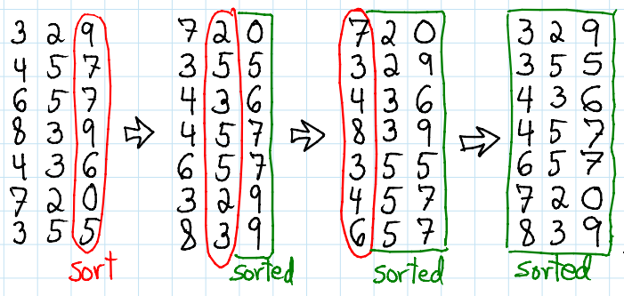
Source: https://brilliant.org/wiki/radix-sort/

In this example, d equals three and we are in base 10. What if all the numbers don’t have the same number of digits in the chosen base? It is not a problem, d will be the number of digits of the largest number in the list and we add zeros as digits at the beginning of other numbers in the list, until they all have d digits too. This works because it doesn’t change the value of the numbers, 00256 is the same as 256. An example follows.

Radix Sort example with an unequal number of digits for the numbers to sort.
Radix Sort example with an unequal number of digits for the numbers to sort. We fill most significant digits with zeros for the numbers which don’t have as digits as the largest number in the list to be sorted. Here, they all have three digits except 9 which becomes 009.
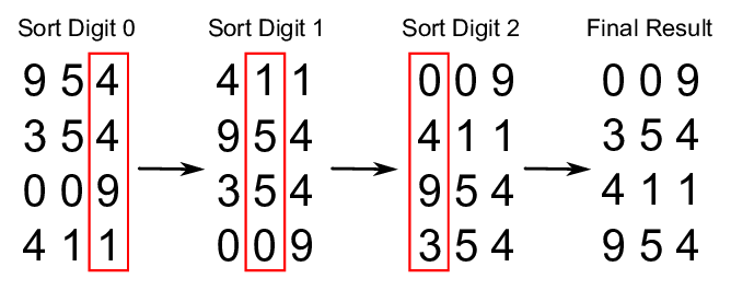
Source: https://github.com/trekhleb/javascript-algorithms/tree/master/src/algorithms/sorting/radix-sort

Keep in mind that we could have chosen any other number base and it will work too. In practice, to code Radix Sort, we often use base 256 to take advantage of the bitwise representation of the data in a computer. Indeed, a digit in base 256 corresponds to a byte. Integers and reals are stored on a fixed and known number of bytes and we can access each of them. So, no need to look for the largest number in the list to be sorted and arrange other numbers with zeros as explained. For instance, we can write a Radix Sort function which sorts int16_t (integers stored on two bytes) and we know in advance (while writing the sort function) that all the numbers will be composed of two base 256 digits. Plus, with templates-enable programming languages like C++, it is straightforward to make it works with all other integer sizes (int8_t, int32_t and int64_t) without duplicating the function for them. From now, we assume that we use the base 256.

Why use counting sort or bucket sort?

First, if you don’t know Counting Sort or Bucket Sort, I highly recommend to read about it and figure out how they work. They are simple and fast to understand but expose and explain them here will make this post too long and it is not really our purpose today. You will find plenty of examples, articles and videos about them on the internet. Sorting algorithms are at least as older as computer science and first computers. They have been studied a lot since the beginning of programmable devices. As a result, there is a lot of them and it is not only good but also important to know the main ones and when to use them. Counting and Bucket sorts are among the most known.

They are useful in the Radix Sort because we take advantage of knowing all the value range one byte can take. The value of one byte is between 0 and 255. And this helps us because in such conditions, Counting Sort and Bucket Sort are super simple and fast! They can run in O(N) when the length of the list is at least a bit greater than the maximum (in absolute value) of the list and especially when this maximum is known in advance. When it is not known in advance, it is more tricky to make the Bucket sort runs in O(N) than the Counting. However, in both cases, the maximum and its issues have to be managed dynamically. They can run in O(N) because they are not comparison-based sorting algorithms. In our case, we sort according to one byte so the maximum we can have is 255. If the length of the list is greater than 255, which is a very small length for an array, Counting and Bucket sorts in Radix Sort, can easily be written having O(N) complexity.

Why not use only either counting or bucket sort to sort the list all of a sudden? Because we will no longer have our assumption about the maximum as we are no longer sorting according to one byte. And in such conditions, the complexity of Counting sort is O(N+k) and Bucket sort can be worse depends on implementations. Here, k is the maximum number of the list in absolute value. In contrast, with Radix Sort, you will have in worst case O(8*N) which is O(N) and we will explain why. In other words, since Radix Sort iterates through bytes and always sorts according to the value of one byte, it is insensitive to the k parameter because we only care about the maximum value of one byte. Unlike both the Counting and Bucket sorts whose execution times are highly sensitive to the value of k, a parameter we rarely know in advance.

The last point of why we use them in Radix Sort is because they are stable sorts and Radix Sort entirely relies on stability. We need the previous iteration output in the stable sorted order to do the next one. No better way to try it by yourself quickly on a paper sheet with a non-stable sort to understand why. Actually, you can use any stable sorting algorithm with a complexity of O(N) instead of them. There is no interest in using one with a complexity of O(N log(N)) or higher because you will call it d times and in such a case, it is just worse than call it once with the entire numbers to sort them all of a sudden.

Complexity of Radix Sort

The complexity is O(N*d) because we simply call d times a sorting algorithm running in O(N). Nothing more. The common highest integer size in a computer is integer on 8 bytes. So assuming we are dealing with a list of integers like that, the complexity using Radix Sort is O(8*N). The complexity will be lower if we know that they are 4 or 2 bytes integers as d will equal 4 or 2 instead of 8.

LSD VS MSD Radix Sort

The algorithm described above is called LSD Radix Sort. Actually, there is another Radix Sort called MSD Radix Sort. The difference is:

  • With the LSD, we sort the elements based on the Least Significant Digit (LSD) first, and then continue to the left until we reach the most significant digit
  • With the MSD, we sort the elements based on the Most Significant Digit (MSD) first, and then continue to the rigth until we reach the least significant digit

The MSD Radix Sort implies few changes but the idea remains the same. It is a bit out of our scope for today so we will not go in further details, but it is good to know its existence. You can learn more about it here.

How can Radix Sort be useful to gain speedup?

The Radix Sort is not so often used whereas well implemented, it is the fastest sorting algorithm for long lists. When sorting short lists, almost any algorithm is sufficient, but as soon as there is enough data to sort, we should choose carefully which one to use. The potential time gain is not negligible. It is true that “enough” is quite vague, roughly, a length of 100 000 is already enough to feel a difference between an appropriate and an inappropriate sorting algorithm.

Currently, Quicksort is probably the most popular sorting algorithm. He is known to be fast enough in most of the cases, although its complexity is O(N log(N)). Remember that it is the lower bound for comparison-based algorithms and the Radix Sort has a complexity of O(N*d). Thus, Radix Sort is efficient than comparison sorting algorithm until the number of digits (d parameter) is less than log(N). This means the more your list is huge, the more you should probably use the Radix Sort. To be more precise, from a certain length, the Radix Sort will be more efficient. We know the Radix Sort since at least punch cards era and it can do much better. So why it is not so used in practice?

Typical sorting algorithms sort elements using pairwise comparisons to determine ordering, meaning they can be easily adapted to any weakly ordered data types. The Radix Sort, however, uses the bitwise representation of the data and some bookkeeping to determine ordering, limiting its scope. Plus, it seems to be slightly more complex to implement than other sorting algorithms. For these reasons, the Radix Sort is not so used and this is where my project comes into play!

My project

My project is to implement a reusable C++ library with a clean interface that uses Radix Sort to sort a distributed (or not) array using MPI (if distributed). The project focus on distributed arrays using MPI but the library will most probably also have a serial efficient version of Radix Sort. The goal is that the library allows users to sort any data type as long as they can forgive a bitwise representation of their data. If the data are not originally integers or reals, they will have the possibility to provide a function returning a bitwise representation of their data.

Challenge

The time has come to make the announcement! I will soon launch a challenge, with a gift card for the winner, which simply consists in implementing a sorting algorithm that can sort faster than mine, if you can… A C++ code will be given with everything and a Makefile, your unique action: fill in the sorting function. Open to everybody, the only rule: be creative. Can you defeat me?

All information concerning the challenge in my next blog post so stay tuned! I am looking forward to tell you more about it.

See you soon

To be honest, this post should have been written before the previous one. But as they say, better late than never.

If the previous post consisted of describing the theoretical principles behind an aerodynamics simulation, this one is going to deal with the actual user-level experience of doing it in a supercomputer. Again, the aim is that absolutely anyone that ends up in this post is able to understand what I am writing about. Feel free to drop a comment if something is not clear enough.

From now on, let’s assume that, by whatever reason, you have been given the opportunity to use a supercomputer. The post is going to be about how the experience would be, and what you would have to do in order to be able to use it, as opposed to a regular computer.

How do I turn it on?

That is indeed a logic question. When you want to use your personal computer, the first thing that you have to do is to push the on/off button. However, things work completely differently in that respect in a supercomputer. A supercomputer is always on.

As I said in the previous article, one can think of a supercomputer as a regular computer that features many more processors, much more RAM and, eventually, a much bigger size. But there are many other differences that I purposely omitted last time.

To begin with, a supercomputer is so large that it is rarely used just by one user at a time. Typically, many different users are connected to it, performing completely independent tasks. And the word connected is highlighted because it is very relevant: you do not physically use the supercomputer, bur rather you remotely connect your computer to it: you gain access to it by typing an address (a username) and its associated password, and then you can use it from your computer as if you were using your own computer. For you, the supercomputer will be just one more window in your computer. With the key difference that the simulations that you will run will not be physically run by your computer (i.e. you will not hear the sound of the fans revving up). They will be integrally run in the supercomputer, which may be on the other side of the wall, or thousands of kilometres away from. For those of you who have already connected to another computer via Team Viewer, this concept will be more familiar.

The as if you were using your own computer sentence is also a little optimistic and, essentially, inaccurate. There will indeed be some major differences, especially from a Windows-user perspective.

The most intuitive difference will be that, in the first instance, you will not be able to access the files and the programs that are installed in your personal computer when you are in the supercomputer window. So if you want to make use of some of your PC/laptop files in the supercomputer, you will have to find a way to transfer them. Of course, there are easy solutions to accomplish that task. But is something that must be kept in mind: even if you see the supercomputer just as a window opened in your computer, it is not possible to do things like dragging and dropping files into it. It is still a different computer.

Windows? What is that?

The other key difference (and this is why I mentioned the Windows-user perspective aspect above) is that the vast majority of supercomputers run Linux instead of Windows or any other operating system, for a variety of reasons (customizability, licensing or potential users knowledge). So if your PC runs Windows and you have never used Linux, this also constitutes a great difference.

Screenshot of my login running session in the Salomon supercomputer, taken at the very moment I was writing this post. Own elaboration.

Of course, Linux is far from being something exclusive of supercomputers, and this post is not intended to describe the differences between Windows and Linux. But still, I think that a general view of how to deal with a supercomputer cannot be provided without saying something about Linux.

When working with Linux, the most efficient way of navigating through the computer and to perform tasks is not by making use of a mouse and double-clicking in icons, which is the conventional way of working in Windows. In Linux, once you are connected to the supercomputer, you enter into the folders or into the files by writing commands in the terminal, something that is represented in the image above. For example, if we are on the desktop, we can type ls and hit enter, and we will get a list of folders and files out there, even if we cannot see them directly. And if we want to enter a folder, we will write cd + name of the folder and hit again enter, instead of double-clicking on the folder. ls and cd are just two of the many commands that make that, once dominated bash and the shell (which can be said to be the language and the internal program on which all this is based), working in Linux is very efficient.

Another different question is how one can connect to a Linux-based supercomputer from a Windows-based personal computer, which is often the case. However, this is something more difficult to explain than to actually do and does not add much value to the post, so it will be set aside on this occasion.

I want to use a supercomputer. Is this possible?

Yes, you can use a supercomputer if you want. But you have to truly want it, which means that you have to present a project that is deemed to be worthy of those resources. If you are successful, you will be provided with a given amount of core hours, which basically represent the amount of time that you can make use of the supercomputer. The actual time will depend on how many of its processors you use (that is the reason why the time is distributed in core hours and not simply in hours of usage).

For example, the European computers that belong to the PRACE network periodically hold a contest in which the available core hours of the supercomputer for a period of time are assigned to the best projects. In particular, the rules applying to the current contest for the supercomputers’ resources here in Ostrava can be found here.

What happens if the supercomputer is overcrowded?

Since the core hours are distributed among the users only once every several months, the users have a fair amount of freedom to choose when to make use of the supercomputer. It may happen that, suddenly, many users want to work with the supercomputer at the same time. This is something that happens from time to time, and in fact, it was happening at the moment in which I took the image above (the capital Q’s that mean that the simulations that I want to run are in the queue, waiting for others to finish).

This issue is so important, that there is a whole world of investigation around it. Because, how do we decide which user should hold preference when using the supercomputer? In order to make it as fair as possible, complex algorithms (called job scheduling algorithms) are implemented to distribute the time among the users in an appropriate way, taking into account factors such as how much time has that user already consumed, how long will their simulations take, etc. A very nice introduction to this topic was provided by one of last year’s Summer of HPC participants in its final presentation.

Conclusions

The objective of this post was to make you imagine how it would be to use a supercomputer, specially in the case that it is a situation you will never face in your life. I do not know what level of immersion I have reached, but at least I hope this will be useful for you to have a rough idea of what this world is about. Next time, when people tell you about supercomputing, you can answer: “Hey, you are not going to impress me with that. I know what you are talking about!”.

——————————————————————————————————–

Ahora, ¡en español!

¿Cómo se usa un superordenador?

Siendo honesto, este post debería haber sido escrito antes que el anterior. Pero más vale tarde que nunca.

Si el post anterior consistía en describir los principios teóricos de una simulación aerodinámica, este va a tratar sobre la experiencia real de hacerlo en un superordenador a nivel de usuario. Una vez más, el objetivo es que cualquier persona que acabe en este post sea capaz de entender de lo que estoy escribiendo. Siéntete libre de escribir un comentario si algo no está lo suficientemente claro.

De ahora en adelante, supongamos que, por cualquier razón, te han dado la oportunidad de usar un superordenador. El post va a ir sobre cómo sería la experiencia, y qué tendrías que hacer para poder usarlo diferente de lo que harías en un ordenador normal.

¿Cómo lo enciendo?

Esta es una pregunta bastante lógica. Cuando uno quiere utilizar su ordenador personal, lo primero que tiene que hacer es pulsar el botón de encendido/apagado. Sin embargo, las cosas funcionan de forma completamente diferente en un superordenador. Un superordenador siempre está encendido.

Como dije en el artículo anterior, uno puede pensar en un superordenador como un ordenador normal que cuenta con muchos más procesadores, mucha más RAM y, en definitiva, un tamaño mucho mayor. Pero hay muchas otras diferencias que omití a propósito en el último post.

Para empezar, un superordenador es tan grande que rara vez es utilizado por un solo usuario a la vez. Lo normal es que muchos usuarios diferentes estén conectados al mismo tiempo, realizando tareas completamente independientes. Y la palabra conectados está resaltada porque es muy importante: el superordenador no se utiliza físicamente, sino que el usuario se conecta a él de forma remota: se accede a él escribiendo una dirección (un nombre de usuario) y su contraseña asociada, y se utiliza desde el ordenador personal. Para ti, el superordenador será sólo una ventana más en tu ordenador, con la diferencia clave de que las simulaciones que se ejecutarán no serán ejecutadas físicamente por el ordenador (es decir, no se oirá el sonido de los ventiladores de tu ordenador acelerando). Se ejecutarán integralmente en el superordenador, que puede estar al otro lado de la pared, o a miles de kilómetros de distancia. Para aquellos que ya se han conectado a otro ordenador a través de Team Viewer, este concepto será más familiar.

La frase como si estuvieras usando tu propio ordenador es un poco optimista y, esencialmente, inexacta. Realmente, habrá algunas diferencias importantes, especialmente desde la perspectiva del un usuario acostumbrado a Windows.

La diferencia más intuitiva será que, al principio, no podrás acceder a los archivos y programas que están instalados en su ordenador personal cuando estés en la ventana del superordenador. Por lo tanto, si quieres utilizar algunos de los archivos de tu PC/laptop en el superordenador, tendrás que encontrar una forma de transferirlos. Por supuesto, hay soluciones fáciles para llevar a cabo esa tarea. Pero es un ejemplo de algo que hay que tener en cuenta: incluso si se ve el superordenador como una ventana abierta en el ordenador, no es posible hacer cosas como arrastrar y soltar archivos en él, o copiar y pegar sin más. Sigue siendo un ordenador diferente.

¿Windows? ¿Qué es eso?

La otra diferencia clave (y es por esto que mencioné el aspecto de la perspectiva del usuario de Windows arriba) es que la gran mayoría de los superordenadores están bassados en Linux en en vez de en Windows o cualquier otro sistema operativo, debido a diferentes motivos (capacidad de personalización, licencias o conocimiento de los usuarios potenciales). Por lo tanto, si tu PC está basado en Windows y nunca has utilizado Linux, esto también constituirá una gran diferencia entre usar tu ordenador habitual y usar un superordenador.

Captura de pantalla de mi sesión conectado al superordenador Salomon, tomada mientras escribía este post. Elaboración propia.

Por supuesto, Linux está lejos de ser algo exclusivo de los superordenadores, y este artículo no pretende describir las diferencias entre Windows y Linux. Pero aun así, creo que no se puede dar una visión general de cómo tratar con un superordenador sin hablar un poco sobre Linux.

Cuando se trabaja con Linux, la forma más eficaz de navegar por el ordenador y realizar tareas no es utilizando el ratón y haciendo doble clic en los iconos, que es la forma convencional de trabajar en Windows. En Linux, una vez conectado al superordenador, se entra en las carpetas o en los archivos escribiendo comandos (líneas de texto) en la terminal, algo que está representado en la imagen de arriba. Por ejemplo, si estamos en el escritorio, podemos escribir ls y darle al enter, y nos aparecerá una lista de las carpetas y archivos que hay, aunque no los podamos ver directamente. Y si queremos entrar en una carpeta, escribiremos cd + nombre de la carpeta y le daremos al enter, en vez de hacer doble click encima de la carpeta. ls y cd son solo dos de los muchos comandos que hacen que, una vez dominado bash y la shell (que digamos que son el lenguaje y el programa interno en el que todo esto está basado), trabajar en Linux sea muy eficiente.

Otro tema diferente es cómo es posible conectarse a un superordenador basado en Linux desde un ordenador personal basado en Windows, que suele ser el caso. Sin embargo, eso es más difícil de explicar que de hacer y no añade mucho valor al post, por lo que se esta vez no voy a hablar de ello.

Quiero usar un superordenador. ¿Es posible?

Sí, puedes usar un superordenador si quieres. Pero hay que querer de verdad, lo que significa que hay que presentar un proyecto que se considere digno de esos recursos. Si tienes éxito, se te proporcionará una cantidad determinada de horas de procesador, que básicamente representan la cantidad de tiempo que podrás hacer uso del superordenador. El tiempo real que puedas usarlo dependerá de cuántos de los procesadores del superordenador utilices (esa es la razón por la que el tiempo se distribuye en horas de procesador, y no simplemente en horas de uso).

Por ejemplo, los ordenadores europeos que pertenecen a la red PRACE celebran periódicamente un concurso en el que las horas de procesador disponibles en el superordenador durante un período de tiempo se asignan a los mejores proyectos. En concreto, las reglas que se aplican al concurso para los recursos de los superordenadores aquí en Ostrava se pueden encontrar en este enlace.

¿Qué ocurre si demasiada gente quiere usar el superordenador a la vez?

Dado que las horas de procesador se distribuyen entre los usuarios solo una vez cada varios meses, los usuarios tienen una gran libertad para elegir cuándo hacer uso del superordenador. Puede ocurrir que, de repente, muchos usuarios quieran trabajar con el superordenador al mismo tiempo. Esto es algo que sucede de vez en cuando, y de hecho, estaba sucediendo en el momento en que tomé la imagen de arriba. Las cus mayúsculas (Q) significan que las simulaciones que quiero ejecutar están en la cola, esperando a que otras terminen.

Este tema es tan importante que hay todo un mundo de investigación a su alrededor. Porque, ¿cómo decidimos qué usuario debe tener preferencia a la hora de utilizar el superordenador? Para que sea lo más justo posible, se implementan unos algoritmos complejos (llamados algoritmos de planificación de tareas) para distribuir el tiempo entre los usuarios de forma adecuada, teniendo en cuenta factores como el tiempo que el usuario ya ha consumido, el tiempo que tardarán sus simulaciones, etc. Una introducción muy interesante a este tema fue dada por uno de los participantes del Summer of HPC del año pasado en su presentación final.

Conclusiones

El objetivo de este post era hacerte imaginar cómo sería usar un superordenador, especialmente en el caso de que sea una situación que no ocurrirá en tu vida. No sé si he conseguido un gran nivel de inmersión, pero al menos espero que te sirva para tener una idea aproximada de lo que es este mundo. La próxima vez, cuando la gente te hable de supercomputación, puedes responder: “Oye, no te creas que me vas a impresionar con eso. ¡Sé de lo que hablas!”.

So… Remember the test environment setup I was working on last time? I had to drop it last week. The PCOCC installation took me some time and a lot of patience, but it did run through at the end. Unfortunately, I was already a bit behind my schedule when that happened, and when I couldn’t start up a cluster of virtual machines with it within a few days, it definitely threw me out of my time window. Time to find a new approach…

As frustrating as dropping everything I had worked on for 3 weeks might be, these things can happen. It’s holiday season, a lot of people are out of the office, and everyone who stays behind is busy because they have to deal with the work left by those on leave. In my case, there was only very few colleagues with the technical knowledge about PCOCC and all the tools beneath it required for my setup, the documentation linked by PCOCC is a bit outdated and it doesn’t seem to have a big user base (no really, when you google “PCOCC”, the fifth result is my project description). I also didn’t have access to the SURFsara documentation about their PCOCC setup and only a regular user account on Cartesius, so I couldn’t look at all the configuration details there either. And that is how it came that I spent half a day doing git-diffs on different versions of SLURM to find out which would be compatible with a plugin needed. At the end, due to the narrow time frame of this project, it didn’t make sense to continue working on the test environment for more then half of my time here.

Luckily, my mentor returned from holiday last Wednesday so we could talk it through and he proposed I instead set up a virtual machine with KVM, the Linux hypervisor, and libvirt, a virtualization API, and add an encrypted disk to it. This will act as a proof of concept for HPC with encrypted disks and as a basis for some benchmarking. If you’re interested in some technical details, I’ll describe those in another blog post!

Of course not, but I have input for benzene and I did the first tests of the electron density computation on this system. Before showing the results (Pretty figures!), I would like to tell you about the helical symmetry (something that makes the computation faster) and give some insight into the nanotube code.

Helical symmetry of nanotubes

Tyger Tyger, burning bright, 
In the forests of the night; 
What immortal hand or eye, 
Could frame thy fearful symmetry? 

William Blake: The tyger

Symmetry is something that is pleasing for human eye in general, and it has an important role in chemistry as well. The symmetry of molecules is usually described by point groups that contain geometric symmetry operations (mirror plane, rotational axis, inversion center). For example, the water molecule belongs to the C2v point group: it has a mirror plane in the plane of the atoms, another one at the bisector of the bond angle, and a twofold rotational axis, and the identity operator. (I shall note that there is another way to describe the symmetry using permutation of the identical nuclei, which is a more general approach.) Point group symmetry can be used to label the quantum states and it can be incorporated in quantum chemistry programs in a clever way to reduce the cost of the computation.

In my previous post I wrote about how to “make” a nanotube by rolling up a two-dimensional periodic layer of material. The resulting nanotube is periodic along its axis, it has one-dimensional translational symmetry. In the case of a carbon nanotube with R=(4,4) rolling vector the translational unit cell contains 16 carbon atoms (see figure, yellow frame). However, it is better to exploit the helical and translational symmetry (pseudo two-dimensional approach), where the symmetry operation is a rotation followed by a translational step. It this case it is sufficient to use a much smaller unit cell (only two atoms) for the R=(4,4) carbon nanotube. The small unit cell is beneficial because it makes the computation cheaper. The figure below shows the atoms of the central unit cell in red, and the green atoms are generated by applying the rotational-translational operation twice in both directions.

Helical symmetry of the R=(4,4) carbon nanotube

What does the code do?

So, we have a program that can compute the electronic structure of nanotubes (the electronic orbitals and their energies) for a given nuclear configuration. I would like to tell you how it works but I cannot expect you to have years of quantum chemistry study and I don’t want to give you meaningless formulas. Those, who are familiar with the topic can find the details in J. Comput. Chem. 20(2):253-261 and here.

Basis set: Contracted Gaussian basis. The wave function is the linear combination of some basis functions. From the physical point of view the best choice would be using atomic orbitals (s-, p-, d-orbitals), but for a computational reason it is better to use (a linear combination of) Gaussian functions that resemble the atomic orbitals. The more basis functions we use, the better the result will be but the computational cost increases as well.

Level of theory: Hartree-Fock. This is one of the simplest ways to describe the electronic structure. The so-called Fock operator gives us the energy of the electronic orbitals. It is a sum the two terms. The first contains the kinetic energy of the electron, the Coulomb interaction between the electrons and the nuclei, and the internuclear Coulombic repulsion. The second term contains the electron-electron repulsion. The Fock operator is represented by a matrix in the code, and the number of basis functions determines the size of the matrix.

To get the basis function coefficients and the energy we have to compute the eigenvalues of the Fock matrix. To create the matrix we already have to know the electron distribution, so we use an iterative scheme (self consistent field method): Starting from an initial guess, we compute the electronic orbitals, rebuild the Fock matrix with the new orbitals, and diagonalize it again, and so on. The orbital energy computed with an approximate wave function is always greater than the true value, so the energy should decrease during the iteration as the approximation gets better. We continue the iteration until the orbital energies converge to a minimum value. This is how it is done in a general quantum chemistry program, but in our nanotube program it is different, as you will see in the next section.

Transformation to the reciprocal space. The translational periodicity allows us to transform the basis functions from the real space to the reciprocal space (Bloch-orbitals). This way the Fock-matrix will be block diagonal. We diagonalize each block separately, which is a lot cheaper than diagonalizing the whole matrix. This part is parallelized with MPI (Message Passing Interface), each block is diagonalized by a different process.

The results are orbital energies and basis function coefficients for each block. So far the main focus was on the energies (band structure), but now we will something with the orbitals as well.

Finally: the electron density

Now let’s get down to business. The electron density describes the probability of finding the electron at a given point in space, and it is computed as the square of the wave function. Now we are not interested in the total electron density, but the contribution of each electron orbital. For the numerical implementation we have to compute the so-called density matrix from the basis coefficients of the given orbital, and then contract it with the basis functions. First, we compute the electron density corresponding to the central unit cell in a large number of grid points. The electron density of the whole nanotube is computed from the contribution of the central unit cell using the helical symmetry operators.

Let’s see an example, the benzene molecule. (I know it’s not a nanotube, but it’s a small and planar system that is easy to visualize). The unit cell consists of a carbon and a hydrogen atom, and we get the benzene replicating and rotating it six times, and we do the same way for the electron density. This particular orbital shown in the picture is made of the pz-orbital of carbon and the s-orbital of hydrogen. On the left electron density figure, you can see the nodal plane (zero electron density) of pz between the two peaks; and the merging of the pz and the s-orbital to a covalent bond.

Linear combination of atomic orbital to molecular orbital
Generating the electron density of benzene from one unit cell
(Grid points are in the plane of the molecule)

The next steps

Recently I have been testing the parallel version of the electron density computation to see if it gives the same result as the serial code or not. I hope it does, so “parallelization” is not among the next steps. (However, one can always improve the code). The next challenge is the visualization of the electron density in 3D.

This week, I show how I created animations for collective communications and transferred them to Wee Archie (with videos) and introduce the wave simulator. I’ll also talk about issues with my system on Wee Archie and how this will affect my goals going forwards. Make sure not to miss the cute animal pictures at the end!

Animating Collectives

Since my last post, I’ve created a prototype of every type of MPI communication needed for an outreach demonstration. You can see the collective communications in the video below, run on a Wee Archlet. For details on how I made these animations, and what a Wee Archlet is, see the previous post. These aren’t quite the final animations, but are a good proof of concept which I’ll polish as I create the final interface for the demos.

Collective Communications on Wee Archlet

For full context, a collective communication is a one-to-many or many-to-many communication, vs. the simpler one-to-one communications of last post. Some of the most commonly used collectives are shown above. In one-to-many, a master Pi is needed, one which controls the flow, gives out all the data, or receives all the data. Here, this is always the bottom Pi.

Gather will collect data from every computer in your group and drop it all on one. Reduce will do the same, but apply an operation as it goes to the data – here it sums it up. Broadcast will send data from the root to every computer in the group. Scatter will do the same, but rather then send them all everything, they each get slices of the data.

Animating for Production

Once I had finished prototyping my animation server on the Wee Archlet, and created animations for many simple operations, it was time to get it working on Wee Archie. Transferring my animations to render on Wee Archie was easy in theory… It ended up taking less time than I thought it was going to, but there were still many complications that need to be ironed out! Below you can see one of my first demonstrations on Wee Archie.

How would you broadcast a message from one computer to every other one on a network? Would you just get it to send it to them all, one by one, or try and send them all at once? Neither is perfect – what if the message is large, or the network is slow to start a connection on? A different approach to sending these messages is shown below, which is the best way to make full use of network where all the computers are connected to each other, and the actual processing of the message will take a while compared to the sending.

Broadcasting Explanation on Wee Archie

Here, you can see the broadcast as shown earlier, but broken down so you see how it happens inside MPI (a simplified version, anyway). Here, one of the central Pis will send a message to every other one. There are 16 of them, so with the implementation I show, you can do it in 4 steps! Assuming all of your Pis are connected to each other, and all connections are as fast as each other, this is a very fast way of getting a message across.

Initially, the central Pi will send the message to a neighbour. This means the neighbour also has the message, so they can both pass it on! When they do this to their neighbours, now 4 have the message. Then they will all pass on the message to another neighbour, and then we have 8. If there were more, this would continue on, but we’re done after the next step, when the 8 send on their message, and all 16 Pis have it!

This demonstration will be the final one in a series of tutorials building up to it, illustrating the basics of parallel computing on Wee Archie. They include all the previous demos I’ve shown in some form, with explanations and motivation as you go. They’re mostly written now, and when the first version is complete, they’ll all be posted on the Wee Archie Github repository.

The main issue with the current system is lack of synchronisation. Because I use HTTP requests to queue all my animations, they often end up out of sync – starting a connection takes time. A potential fix for this is setting up a network of pipes using WebSockets, which I’ll investigate soon. The other main issue is playback speed – I need a global control for frame rate on the various animations, as well as the ability to change this as the circumstance needs it. Hopefully making this part of the server doesn’t prove too difficult, as it would improve the feel of the animations a lot!

Introducing the Sea

So, the famed wave simulator, or coastline defence simulation – what is it?

Initially developed by my mentor Gordon Gibb, it’s the most recent demonstration for Wee Archie. It asks the user to place a series of coastal defence barriers – represented here by gray blocks. You have a budget, and each block has a fixed cost. The coastline has several different locations pictured. They are more or less susceptible to being damaged, and damage costs various amounts.

For example, the beachfront is cheap and easy to damage. The cliff-top housing is hard to damage and expensive. The library, expensive and easy to damage. The shopping market is somewhere in-between them all.

Wave Simulator (Current Version)

When you place the barriers and set it running, it will run a fluid simulation, and show the waves hitting the shore, calculating the damage they do, and how effective your barriers are! At the end of it, the amount of money saved/spent is your score. It’s quite simple to use, and very popular at outreach venues such as Edinburgh Science Festival.

All the current demonstrations use a framework where Wee Archie runs a server on the access Pi – the left of the two on top in the video. This server will run the simulations when called, and give the data back to the client, a graphical Python application running on the connected laptop.

Upcoming Goals

So this week I’ll be working on getting the wave demo working using my version of MPI, showing the communication as it happens. I won’t be able to show all of them, as to render the simulation, there are hundreds of operations per second, but I’ll display the main logic of the program once or twice out of those hundreds.

The nice thing about visualising communication is that unlike the data in the program, the way the computers communicate stays the same throughout the execution. It also doesn’t need advanced mathematics to understand. This makes it a good thing to sample and explain in detail!

The next goal after this will be to change the graphical interface from Python to running in the browser. Once I set this up, I’ll be able to host a website on Wee Archie, and all the client computer will have to do will be connect! The website will be able to host all the tutorial I write and the demonstrations, and easily include extra details, explanations and resources.

If it goes well and porting over the old demos is fast enough, I anticipate it being the future for Wee Archie. If I have all that working by the end of the project I’ll be very pleased with the progress made, as it will have improved the experience of using Wee Archie enormously. Rather than a collection of independent demos, it can be a cohesive whole which lets students explore at their own pace and learn as they go!

Sightseeing Segment

It’s been a couple of weeks, but it’s been very busy. I haven’t had time to see too much, though last weekend I visited the beautiful Pentland Hills regional park. The swan featured in this post is from the reservoir there in Glencorse. It’s a beautiful park, with many options for different visitors, though I stuck to some trekking through the fields – getting a bit sunburned in the process. I hope to go swimming in the reservoir with the others if the weather holds!

Swan in Glencorse Reservoir

Sadly, I am not much better at ping pong then I was previously. I don’t think I was cut out for this line of rapid reflex wrist-flicking work. I’ve managed to take one game off Benjamin, but it was in the face of many! I hear the Fringe has some public tables which are better than the one in our accommodation, so perhaps that will help?

I spent the first few weeks at Computing Centre of the Slovak Academy of Sciences getting familiar with the nanotube code. We actually changed the goal of the project a bit. The original plan was the further development of the MPI parallelization, but now I am working on an extension of the code with a new feature. The task is to compute (and visualize) the electron density of the orbitals that come out of the simulation.

In this blog post, I am giving a short introduction to quantum chemistry in general, and I will tell about the interesting things I have learnt about nanotubes.

How to make a nanotube in 3 easy steps

Due to their extraordinary properties, nanotubes are in the focus of material science, nanotechnology and electronics as well. Carbon nanotubes are cool things indeed: they are one of the strongest materials, they can behave either like metals or semiconductors, they have good thermal conductivity, and they are the material of Vantablack, too.

You can make a nanotube this way in a thought experiment (the real synthesis is not this, of course):

  • Step 1: Take a layer of a two-dimensional periodic material, for example, a sheet of graphene. Periodicity means that you can construct the whole material by translating a repetitive unit, the unit cell. In the picture, the unit cell (blue) contains two carbon atoms, and has two unit vectors.
  • Step 2: Define the rolling vector (purple) by connecting the centers of two unit cells of the graphene sheet. Cut out a rectangle whose one side is the rolling vector.
  • Step 3: Roll up the nanotube by connecting the two ends of the rolling vector.

Congratulations, now you have a carbon nanotube!

This is how we can imagine making nanotube from a graphene sheet.

Its material and the rolling vector characterize the nanotube. The rolling vector determines the diameter, the structure (armchair, zigzag or chiral), and the conductivity (metallic or semiconducting).

Nanotubes with different rolling vectors

Quantum chemisty in a nutshell

The potential engineering applications made the nanotubes an important topic of computational science. I am working on a code that computes the electronic structure of the nanotube. But before going into details about the particular code, I would like to tell you about quantum chemistry in general.

Some people, who asked me about my field within chemistry, were really surprized when I told them I am not working in a laboratory, but I am doing computer simulations. They were thinking that chemistry is only about boiling colorful liquids in flasks and experimenting with explosives. But it is not true, at least for the last few decades, the age of computational quantum chemistry. Applying quantum mechanics for molecular systems helps us to explain many experimental phenomena: Why can the matter absorb light only at certain wavelengths? Why can two atoms make a bond? What is the mechanism of a chemical reaction on the molecular level?

The first step to answer these questions is to solve an eigenvalue-equation. In quantum mechanics, we always solve eigenvalue-equations, because physical quantities are described by operators whose eigenvalues are the possible values of the physical quantity, and the quantum states are described by the eigenvectors. The Hamiltonian operator is the operator of the energy, and its eigenvalue-equation is the famous Schrödinger-equation.

Unfortunately, the Schrödinger-equation can be solved analytically only for simple (model) systems, for more complicated cases we do it numerically using computers. How is it done in practice? The wave function will be the linear combination of some basis functions and the Hamiltonian is represented by a matrix. Then, we diagonalize the matrix to get the basis expansion coefficients and the energy.

Goal: Electron density of the nanotube

So, we have the nanotube code that computes the energy of the electron orbitals. My task is to construct the orbitals and the electron density from the basis function coefficients. Electron density tells us the probability of finding the electron at a given point. This way we can visualize the chemical bonds and the nodes of the orbitals. Now, I am working on the serial code and testing it on simple systems like benzene, and I get plots like the one below.

Testing the code: Electron density for one orbital of benzene. White areas indicate high values.

This is enough for now maybe, I will write about the nanotube code and how we do the electron density computation (and hopefully some results) in the next blog post.

In my previous blog post, I discussed the advantages of containerisation when it comes to reproducibility. In short, if you package all of the tools necessary to run your experiments, you can ensure that in future, folk can rerun your systems with minimal hassle.

Since then, I have got access to an HPC system within the Barcelona Supercomputing Center. There, the current design of Docker does not really work, as it requires root access. In a large shared HPC system, granting root permissions to every Tom, Dick, and Perry is not best practice for security, or scheduling fairness.

Thus, I had to look for an alternative. I needed a process of containerisation which would support a shared HPC system, including it’s workload management system such as LSF or SLURM. It should also be easy to integrate with my work so far.

Enter “Singularity

A containerisation system that is HPC-first. Until it was recommended by one of the BSC sysadmins, I had never heard of it before. It integrates well with existing Docker work, allowing you to import existing Docker images, as well as making Singularity-native ones. It also offers a number of domain specific advantages.

In this post, I will walk through a minimum working example of creating a Singularity based experimental workflow.

On our HPC system, we will not have root access. However, the creation of images, and processes such as the installation of packages generally does. Thus, in Singularity one should build and debug images locally, and then copy them over to the HPC system for execution. When testing, you should be sure that your experiments can run without root access, and be wary of where output files are written to.

This a post for people who just want to be able do the following:

  1. Build their code in a container, for reproducibility.
  2. Run that code on a HPC system, for which they don’t have admin privileges.

It contains all of the information I wish I had in one place when I started this work.

Singularity and containerisation is a massive topic, so I will focus on a small workflow. For more complete descriptions of each feature, I advise you use the official docs.

Requirements:

Building Singularity

First, you need to install Singularity locally (somewhere you have root access):

git clone https://github.com/singularityware/singularity.git
cd singularity
git fetch --all
git checkout 2.6.0
./autogen.sh
./configure --prefix=/usr/local
make
sudo make install

Building our first image

To describe and build our container, we use a simple text-file, which we will call the “container recipe”.

Here, you define:

  • The base image to use for your image (e.g. Debian, Ubuntu, Alpine, some other operating system, or even a more fully developed image that you want to build on top of).
  • The files you want to copy into the image.
  • The setup process, of installing necessary packages, building your code, etc.
  • The different “apps”, or “run scripts”, you want your container to perform. For example, your container could have a couple of different experiment modes that could be run. This provides a simple front-end for users of your container.

If you look at mwe.def, you will see we use the Debian Docker base image:

Bootstrap: docker
From: debian:latest

We then copy a number of directories to /root/, including our application code:

%files
    setup /root/
    application /root/
    run /root/

When these directories have been copied, we run our setup and build scripts:

%post
    bash /root/setup/setup_script.sh
    bash /root/setup/build_app.sh

You can see in the scripts ([1], [2]) that we install some packages, move some files around, and compile our code.

Let’s build our image!

sudo singularity build --sandbox mwe.img mwe.def

You’ll notice that instead of images being stored in /var/lib like Docker, you will have all of your files dumped into your working directory. That’s how it is. Plan your .gitignore‘s accordingly.

When we are designing our experimental workflow, it is natural to make changes, and explore what sequence of commands are needed to get things working. Thus, on your local machine, you will want to build sandbox images (notice the --sandbox flag we used. This means that you can connect to the container’s shell, and figure out what commands you need to run in the workflow.

sudo singularity shell mwe.img

These changes are ephemeral by default, which is good. Any packages you install, or build commands you issue which you are happy with should by added to your container recipe.

Run Scripts

When you’re running your experiments, it’s usually simpler to invoke things with a single script, and specify an output directory for results. Issuing the same 14 commands every time is just busy work.

Personally, I recommend at least having a “quick script”, and a “full script”. The quick script should be a minimal version of your experiment, and ideally finish in a short period of time (hence “quick”). The purpose of this is not to collect data, but to test that your experimental workflow is working correctly.

Like Docker, Singularity supports this with the run flag. You can get the default run behaviour of a container with:

singularity run mwe.img

In mwe.def, I have set this to print our run options for this container.

%runscript                                                                                
    exec echo "Try running with --app quick_run|full_run, and specify an output directory"

For example, to run our quick experiment, run like so:

For example, to run our quick experiment, run like so:

singularity run –app quick_run mwe.img ~/results/

Notice that we didn’t need to use sudo for running the container. It is easy to submit this to job processing systems like SLURM and LSF.

In our Singularity recipe, we can define our run options:

%apprun quick_run                           
    exec bash /root/run/quick_script.sh "$@"
                                            
%apprun full_run                            
    exec bash /reprod/full_script.sh "$@"   

The syntax for arguments is the same as normal bash, so $@ represents all arguments, $1 the first, $2 the second etc.

Note that we passed as an argument ~/results. This is a path in our host filesystem outside the container. This is an important point.

By default, your home directory, /tmp, /proc, /sys and /dev filesystems from the host OS are mounted inside the container. So scripts inside the container can write to these locations, with the same permissions of the user. If you run container without root permissions, you will find that most of the file-system will be inaccessible to you. This is by design, which is why you should prefer to have output directories in the auto-mounted directories. You can also manually mount directories, however this is often disabled. See the docs for more information.

Moving to our HPC system

Using the .simg file type, without --sandbox signals to Singularity to make the image a compressed read-only filesystem. This is ideal for our needs, as it reduces filesizes.

Copy mwe.simg to your HPC system. You might want to go for a coffee – even when compressed, containers are not the most space-efficient systems.

You can now try running the quick script, to test things are working. Make sure the Singularity module is activated in the environment, if that’s how your HPC system is set up. Hopefully all is well, and you don’t get any permissions issues. If you do, make sure that your code is not trying to write to any locations that are not mounted, and you have permission to write to.

Finally, we can try the full experiment:

sudo singularity build mwe.simg mwe.def

Try submitting to your HPC system’s job scheduler.

Conclusion

Hopefully this post serves as a good introduction to making reproducible experiments for HPC. You won’t incur much of an overhead running in a container, so I really encourage you to consider doing this more often.

Final things you should consider:

  • how does the architecture of your host machine differ from your target system. Plan compilation flags accordingly.
  • what specific package versions are essential to your experiment? You can’t trust that package repositories will be around forever. If your experiment absolutely needs a particular version of a tool, it is better to download a copy of the package, and install it from file.
  • How are you going to store the project image, and related files? Results can’t be reproduced if people can’t access them.

Dear reader,

I know it has been only a few days since my last post, and I am also aware that you are not used to listening (or maybe reading!) from me so often. However here, at BSC, we are dealing with some minor maintainance experiences that, although “de-energized” part of the network, gave me the chance to think about and report what has been going on the last days.

First and foremost, this week’s highlight has been my visit to MareNostrum 4, i.e. BSC’s supercomputer. Its efficiency and technical characteristics are of course indisputable but what is particularly special about this machine, is also its location. The first image that one faces is that of a 19th-century chapel facade that betrays very little about what’s hidden inside it. Correct! The huge supercomputer which is framed by a glass surface for extra protection is to be found in the interior of this chapel provoking admiration feelings to anyone visiting, no matter how deep an understanding of its use he/she has. This “oxymoron” view that so smoothly combines history with technology can only partially be transferred through the photo below.

MareNostrum 4
Photo:Barcelona Supercomputing Center – National Supercomputing Center (BSC-CNS)/Creative Commons

It is exactly the technology based in this room that allowed me to experiment with the tools and the applications mentioned in my previous post. So, I would say it is about time to jump from this short MareNostrum excursion to the harsh, yet equally interesting, reality!

This reality involves enormous amounts of data that require processing and may come from diverse applications such as those that simulate the movement of billions of air particles or those that attempt to solve rather demanding mathematical problems by deploying computational methods. The behaviour of such applications resembles the one of a wider range of scientific applications, therefore the extracted conclusions can be effortlessly generalized and therefore this is the exact nature of the programs I analyzed!

Valgrind: an instrumentation framework for building dynamic analysis tools. Valgrind tools can automatically detect many memory management and threading bugs, and profile your programs in detail.

But what do I mean by “analyzed”. Well, in order to make that clear we have to take a deeper dive into the different application profiling techniques: Internet is brimming with tools that allow an easy way (sometimes not that intuitive however) to gain insight into an application’s performance and determine the limiting factors. Valgrind is an open-source tool which many of you might know as memory-leak detector, but, believe me, you’d be amazed by the variety of add-on tools that come with it. One of these tools can track down every memory access and determine the number of last-level cache misses. It was this exact tool that was modified in order to perform sufficient sampling rather than give exact memory access numbers.

Sufficient is the keyword! Last week I succeeded in determinig the ideal application-based sampling period that minimizes the experiment execution time, yet provides results which drive in a final performance-enchancing memory data distribution! This would’t have been possible unless the the experimentation process was automated exploiting bash scripts that finally did the work for me! What is not clearly stated here is that I was called to dust off my bash programming skills which remained idle for the last couple of years.

Having obtained results from both benchmark applications what is more is to compare and find a connection between them as well as to correlate the final memory distribution and speedup to the one achieved by hardware implemented profiling. If you are interested in keeping up with the sequel of this story ( I am sorry but not with the Kardashians!) please stay tuned. To be continued…

Don’t forget to check my LinkedIn account for more information.

Hello everyone,

The summer of HPC program is a nice way to discover new countries and place, and before talking a bit more about my actual work here in the next blog post I would introduce you to Jülich and its surrounding.

One of the first thing we get arriving at the laboratory (the so called Jülich Forschungszentrum) was a bike to get from the guest house in the city center to the office. What is very nice is that we can also use it to discover the region, and that is very easy because there is a lot of bike path.

The bike lent by the laboratory.

The city of Jüelich

Jüelich has a very strong historical past, which is still visible in the city we see nowadays, with its iconic citadel from Renaissance and the Napoleonic fortifications. There is a small museum in the citadel, but unfortunately everything is in German. The Napoleonic wall however is inside the Brueckenkopf park, a pleasant place which also host a zoo. All around the city I found a lot of raspberries, that quickly became marmalade and then a pie !

Die Sophienhöhe

Die Sophienhöhe is an hill created by the dirt that was remove from a nearby coal mine, and is now full of vegetation and animals. Since the rest of the region is quite flat, going there offers a cool landscape over all the surroundings.

Lakes around Jüelich

The region of Jüelich is very rich in natural and artificial water plan (because of the Rhur river and the mining activity).
On week-ends, one can take their bike and choose the lake they want to bath in ! We visited two lakes so far : a very wild one where we were almost alone in Barmen, and a more touristic one with more infrastructures, the Blausteinsee.

I hope you liked this guided tour, see you soon for new adventures !

As promised, this is the picture of the house I am living in right now. Pretty good, right? Not as good as it seems though as I do not have air-conditioner in the house!!! I have to live in the hot weather of Italy only with a fan!

As for my project, wonder what I am doing right now? I was initially assigned to work on the simulation of diesel engine. However, due to the confidentiality of the content, the object was changed from diesel engine to airfoil. Even so, it does not really matter much because the purpose of my research is to study the scalability of Paraview Catalyst. One may ask what is Paraview Catalyst? Let me break it down for you. Paraview is basically a post-processing tool for scientific simulation. It allows scientists to view the result of simulations. Remember I told you in the last blog about the colourful airflow animation around an airplane. Yes, you are right, you can do that in Paraview. The picture at the bottom is what I did using Paraview. It may not be obvious but there are two small airfoils inside the colourful “filter-shaped” object. Catalyst is just a feature of Paraview that allows scientist to view the result while running the simulation. It may not sound like a big deal but it can significantly reduce the time for post-processing. Traditionally, post-processing consumes a huge amount of time due to the slow data transfer between processor and storage. Another benefit of Catalyst is it allows scientists to identify the errors while carrying out the simulation.

Currently, I am still working on my project. My aim is to determine whether the benefit of using Catalyst will increase or decrease when the number of processing power increases. This is done by running a lot of simulations and plotting a number of scaling graphs. Curious about the result too? Stay tuned!!!

A month has passed since my stay in IT4Innovations started. Apart from working on my project, which I will comment on below, I’ve been spending my weekends exploring Ostrava and some nearby cities.
The first weekend started with a bang at Colours of Ostrava, where tons of famous bands like The Cure and Florence + the Machine performed at one of the most important music festivals in the Czech Republic. It took place in an old factory, an amazing location full of pipes, huge rusty towers and iron furnaces.

Colours of Ostrava

Another highlight of these weekends has been meeting up with fellow summer of HPC members in Vienna. We stayed for less than two days. We saw an awful lot of palaces, music-related museums (like Mozart’s house) and beautiful gardens. I left eager to come back and continue exploring a city that’s full of history and stories.
Anyways, a month working on my project has given me time to explore and learn a lot about the topic I’m working on. It took a while to get used to all the technology I had to learn, like how to deploy apps on the Movidius Compute Stick or understanding how to use the deep learning frameworks –Keras and Tensorflow.

However, I now feel confident to explain what I’ve been doing, so I will start by giving an overview of the problem I’m trying to solve here, as it drifted away from the original proposal.
I originally was going to address the problem of navigation of urban spaces for blind individuals. In more detail, I was going to train a deep neural network to perform object detection on common obstacles that a visually impaired individual might encounter.
However, after looking deeper into the problem, I found that a big issue that blind individuals face is interacting with newly met people in the street.
None verbal language is a huge part of any social interaction and it can be hard to understand the intent of someone we just met from only the tone of their voice.
So I wondered, what if I could come up with a model able to identify someone’s facial expressions from a video stream? This would make up for a missing visual context and enhance communication for visually impaired individuals.


Once I decided on the new problem I wanted to solve I started looking into the literature of emotion recognition. A relatively naive approach and the one I started with was to train a neural network to classify images based on the emotions represented in them. A classical multiclass classification problem. Most of the datasets available provided images classified on the main 7 emotions: anger, fear, disgust, happiness, sadness, surprise and content. The main issue was the variability of each emotion across different subjects and the lack of specificity in the emotions described. Two facial expressions both identified as happy could be dramatically different. This not only made it quite challenging for the neural network to understand the common patterns underlying facial expressions but was also quite limiting in terms of emotion variability.
Thus, after doing some further reading, I found a much more optimal solution. A perfect way to facilitate the training process, while allowing for more variability in the emotions and without increasing the complexity of the problem.
In 1970, Carl-Herman Hjortsjö came up with a way to encode the most common muscle movements involved in human facial expressions using a Facial Action Coding System (FACS). These muscle movements are called Action Units, and combined action units create facial expressions that can be identified with specific emotions.

Sample action units, taken from https://github.com/TadasBaltrusaitis/OpenFace/wiki/Action-Units

To be able to predict the action units present in a facial expression I will be using a deep neural network.
A very common practice used in the domain of neural networks and computer vision is transfer learning. Transfer learning consists of using part of an existing neural network that has been trained to solve a particular problem and modifying certain layers so it’s able to solve a similar but different problem. In the context of image understanding, what you expect to get from the network you are transferring from is the ability to find patterns and features in images. Because these models are used to classify natural images, there are a lot of features common to these, like edges, surfaces and shapes.

In my case, I’ll be doing transfer learning from a very popular convolutional neural network called VGG16, proposed by K. Simonyan and A. Zisserman from the University of Oxford. More specifically, I’ll be using a version of this convolutional neural network that was trained to detect faces in images.
So, I will use part of this network as a feature detector, and on top of that, I will add a few layers that will work as a classifier for the features identified by the lower layers. The classifier’s job will be to predict the Action Units (or set of muscle movements) present in the image. From that, I will layer another classifier, either another neural network or a simpler clustering algorithm. This classifier will predict the emotion underlying the facial expressions given the set of action units.

The architecture of VGG face, taken from http://www.robots.ox.ac.uk/~vgg/publications/2015/Parkhi15/poster.pdf

I hope this served as a general introduction to my project. Stay tuned for the next post, which will come up pretty soon and will go into detail regarding how I chose and preprocessed the data to train the model and how exactly I modified VGG16 to fit my target problem.

0 Setup

Picture this.
It’s 7 a.m. in the morning. Nobody speaks.
You just woke up.
You unpleasantly turn the lights on.
You do your personal hygiene and other morning routines.
You sit in kitchen, prepare breakfast, make coffee and pour milk in.
You scroll on your phone.
You tap on a not very user friendly website.
You have hard time navigating in it.
You get bored, so you stand up and leave home to go to work.

During this relatable (?) situation, there are 3 moments that are somehow related to what I do here in the University of Ljubljana.

Stick with me.

1 Lights

1a Lights out

A cat turning on the lights.

The moment you turned on the lights, you pressed a button, you allowed electric current to a bulb, which was received from a cable, and if you follow its lead, you end in a power plant. A place that generates power.

But, with a cost. Either to the environment, the environment or to the environment. Despite that the second is more sustainable than the first and the third more sustainable than the second, all energy generation methods have drawbacks.

You might think that drawbacks are inevitable. We always have to sacrifice something.
Right?

1b spotLight

A spotlight stock image.

What if there is a way to generate power from something trivial like water? A way to generate power

  • like the magician pulls a rabbit from an empty hat
  • like the sun generates heat
  • like Zeus’ lightning bolt generates infinite lightnings
  • like internet creates memes out of nothing.

There is a way that allow us to generate very very large amounts of energy from water molecules (Hydrogen, we don’t need oxygen), and some other atoms (Deuterium).

One of the examples in the list is the actual way, and no, memes are not the answer.

1c sunLight

Sun doesn’t have a cable connected to a power plant. However is always shining and providing energy for poor planets like ours. The cheat sun uses, is called plasma fusion.

In short, if small atoms became very hot (more than 10K K or 9727℃), electrons and nuclear separate, and ions and electrons float all over the place like having a party (this is plasma).
If plasma gets very very hot (more than 100M K or 99999727℃), ions are partying so hard, that after one point they can’t stand partying anymore and are coupling into forming larger atoms in a process called plasma fusion. During this coupling, they are having a fest and they celebrate by releasing energy. Big amounts of energy.

For decades, scientists try to construct a hat from which they are able to pull rabbits. They try to create a new small “sun on Earth” to generate power. They tried and designed a Токамáк machine. By using magnets it makes plasma run in circles very very fast and therefore plasma becomes very very hot, and release very very much energy.

A Токамáк machine stock image.

But it didn’t work as effectively as planned. And one of the problems is what happened when you added milk to your coffee.

2 Pour

2a Pour milk in my coffee

When you add milk to your coffee, you will see a mesmerizing image of milk’s random movement in a damn good coffee.

A damn good coffee cup.

A scientist will call this movement turbulent flow, but why you should care?

2b Pour very very very hot plasma
in my very hot plasma

When plasma is running circles inside Токамáк, the core of plasma is the hottest, while plasma on the outer part is colder. It would be ideal if this hot plasma remained steady on its route and didn’t steer right and left (difficult thing to do when partying hard).
Of course, this is not the case.

The so-called plasma microturbulence, is when the central part, the core of plasma, the heart of the party, possibly the hottest thing on Earth,
moves towards the colder part, the peripheral, the party pooper, possibly the second hottest thing on Earth.
When this happens, the heat is dispensed to the colder parts, no fusion is achieved, the party is over, the dream of limitless energy supply gets distant.

2c Pour some computers in my science

Scientists tried to find out how to control microturbulence. But they couldn’t figure things out in small scale experiments. The sun ought to be bigger. However, it is not an easy task to create a machine that makes a large “sun on Earth” just to perform some experiments with it.

Here comes the computers to save the day. Scientists with some help from some computer people, managed to create simulation tools that by solving known equations, allowed the computer to calculate the level of microturbulence in the plasma of the Токамáк machine given specific plasma and machine parameters. Since the scale should be big enough, enormous computational power is needed, and computers have to work day and night.

Here comes HPCs to save the night. Computers in parallel can perform much better than the conventional computers. Hence, most simulation tools have integrated the ability to run in parallel. With these simulations, scientists might understand how to avoid the microturbulence that causes the party to stop, and then we may not be far from day when we could say…

Here comes the sun

The Beatles, Abbey Road

3 Navigate

3a Navigate among trees

Navigation is very important. If you navigate in a tropical forest, you may need a guide to help you.

Me navigating in a forest in Vienna, without a guide.

However if you navigate in a web browser, needing a guide to help you is devastating enough to make you stand up and leave home to go to work.

3b Navigate among numbers

Scientists also have to navigate. In our story, they have to navigate in the results of the simulation. Thousand calculated numbers have to be translated in plots and schemes, in a humanly interpretative way. However, needing a guide to help you navigate and create these plots can be devastating. And if there is no such guide available it can be devastating enough to make you stand up and leave work to go home.

A free to reuse lots-of-numbers image by re_birf

This is the case for a plasma microturbulance simulation, known as Gyrokinetic Electromagnetic Numerical Experiment or GENE. GENE has a proprietary plugin program for visualizing the results. This program was originally created some decades ago, and the GUI (graphic user interface) is very old-school, buggy and not easy to interpret. In fact, if you search “bad UI”, the top results seem very close to the GUI of this program.

3c Navigate among widgets

This is finally where I come. The reason I am here in Ljubljana, Slovenia for this summer, is using some GENE output files that I ‘ll create, and based on the aforementioned GUI, I will create a modern, customizable, interactive, open-source, well-documented GUI to visualize the results of this simulations.

We are on the middle of this summer project, and I have already managed to read and manipulate all the output files, to create the base for the new GUI using PyQt5, to make some first plots, and travel around Slovenia.

So, what I am trying to do here is that I am trying to help scientists do magic, I try shine on the hat so scientists can easily make rabbits appear from it.

Hello from Luxembourg. If you read my previous post, you may be aware that this is where I’ll be spending my summer as part of the PRACE Summer of HPC programme. The official title for the project I’ll be doing here (at the University of Luxembourg to be precise) is “Performance analysis of Distributed and Scalable Deep Learning,” and I’ll spend this blog post trying to give some sort of explanation as to what that actually involves. However, I’m not going to start by explaining what Deep Learning is. A lot of other people, such as the one behind this article, who know more than me about it have already done an excellent job of it and I don’t want this post to be crazily long.

The Scalable and Distributed part, however, is slightly shorter to explain. As many common models in Deep Learning contains hundreds of thousands, if not millions of parameters which somehow have to be ‘learned’, it is becoming more common to spread this task over a number of processors. A simple and widely used example of this is splitting up the ‘batch’ of data points needed for each training step over a number of processors averaging the relevant results over all processors to work out change needed in each trainable parameter at the end. That last part can cause problems however as, like every other area of HPC, synchronization is expensive and should be avoided if possible. To make things more complicated, a lot of deep learning calculations are very well suited to running on GPUs instead of CPUs, which may add more layers of communication between different devices to the problem. 

Despite being a fairly computationally expensive task Deep Learning seems to be quite a popular way of solving problems these days. As a result, several organisations have come up with and published their own, allegedly highly optimized, frameworks to allow programmers to use these techniques with minimal effort. Examples include Tensorflow, Keras, MXNet, PyTorch and Horovod (see logos above). As these libraries all use their own clever tricks to make the code run faster, it would be nice to have a way of working out which is the most suitable for your needs, especially if your needs involve lots of time on an expensive supercomputer. 

Myself and Matteo (also doing a project in Luxembourg) outside the university

This takes us to the surprisingly complicated world of Deep Learning Benchmarking. It’s not entirely obvious how evaluate how efficiently a deep learning program is working. If you want your code to run on a large number of processors, the sensible thing to do is to tweak some hyperparameters so you don’t have to send the vast numbers of parameters mentioned in the previous paragraph between devices very often. However, while this can make the average walltime per data point scale very well, there’s no guarantee the rate at which the model ‘learns’ will improve as quickly. As a result, there are multiple organisations who have come up with a variety of ways of benchmarking these algorithms. This includes MLPerf, which publishes results “time-to-accuracy” results for some very specific tasks on a variety of types of hardware, DeepBench, which evaluates the accuracy and speed of common basic functions used in Deep Learning across many frameworks, and Deep500, which can give a wide range of metrics for a variety of tasks, including user defined ones, for PyTorch and Tensorflow. There are even plans to expand some these to include how efficiently the programs in question use resources like CPU/GPU power, memory, and energy efficiency.

My project for the summer is to set up a program which will allow me to run experiments comparing the efficiency of different frameworks on the University’s Iris cluster (see picture) and to help cluster users choose the most appropriate setup for their task. Ideally, the final product will allow you to submit a basic single device version of a model in one of a few reference frameworks and which would then be trained in a distributed manner for a short time, with some metrics of the kind described above being output at the end. So far, I’m in the final stages of getting a basic version up and running which can profile run with image classification problems Tensorflow, distributed using Horovod. The next few weeks, assuming nothing goes horribly wrong, will be spent adding support for more Frameworks, collecting more complicated metrics, running experiments for sample networks and datasets, and making everything a bit more user friendly. Hopefully, the final version will help users ensure that appropriate framework/architecture is being used and identify any performance bottlenecks before submitting massive individual jobs.

The University’s HPC group, Matteo and I at our office

I’m doing this work from a town called Belval, near the border with France. While the university campus where I work is the main place of interest here, it’s only a short train ride from Luxembourg city, with various towns in nearby France, Germany and Belgium looking like good potential day trips. From my visits so far, the most notable feature of the city centre is the relatively large number of steep hills and even cliffs (one of which requires a lift to get down). This makes walking around the place a bit slow but at least it means I’m getting some exercise. The one low point of my time here was when heat got a bit excessive in the last week. Irish people are not meant to have to endure anything over 35° and I’m not unhappy that I probably won’t have to again this summer. However, there was a great sense of camaraderie in the office, where the various fans and other elaborate damage limitation mechanisms people had set up were struggling to cope. I imagine it would have been a lot less tolerable if the people around me weren’t so friendly, helpful and, welcoming.  

It was only recently that I realized this experience called SoHPC is already midway through and since it has been almost an entire month that I have been silent I decided to drop a few lines in order to give a heads-up on how my time is rolling. If you want to know how it all started, just click here.

The main BSC administrative building.

Everything started in 2014. That was the time when I transited from a schoolboy to an ambitious student (or as one might say: to an ambitious engineer-in-progress). Around 2000 km away from this transition however my current co-workers and mentors were experimenting in optimising applications that used computing systems with exotic memory architectures. Their results were and still are very promising.

Addressing to my 2014 self I feel more than obliged to explain a few technical insights that shall provide a deeper understanding of what is going to follow:

Talking about applications we are essentially refering to computer programs. In order for a program to “run” on our PC it has to store data and what could be a better place to store data if not our PC’s memory system? The most common memory systems (i.e. the ones your laptop probably has) consist of a very slow Hard Drive, which can store more or less one TB of information (thankfully the GBs era is long over) and a quite fast but relatively small (just a few GBs for a conventional laptop) Read Access Memory (RAM). In this point I have to admit that there are also even faster memory architectures present in every computer which however are not in the programmer’s control and thus shall exercise their right for anonymity for this post (and presumably for the ones that will follow). When a “domestic use” program runs, it needs data that ranges from many MBs to a few GBs and therefore it is able to transfer it to RAM where the access is rapid.

The memory hierarchy of a conventional system consists of 3 basic levels which include the CPU built-in caches (from many KBs to a few MBs), the main memory (a few GBs) and the main storage system (from many GBs to a few TBs).

So far so good, but what happens when this “important” data jump from a handful to hundrends of GBs and the memory-friendly application becomes a memory-devourer (the most formal way would be memory-bound)? This is where things take a turn for the worse; this is where this simple memory architecture does not suffice; this is, finally, where more complicated memory levels with various sizes and lower access time come into play. These memory levels are added not in a hierarchical way but rather in more equal one. To understand the organization we could think of a hierarchical system as the political system of ancient Rome, where patricians would be fast-access memory systems that host only the data accessed first (high-class citizens) while plebeians would be slow-access memory systems that host every left data. On the other hand, a more democratic approach, such as the one of ancient Greece, would give equal oportunities to all citizens which in our case would be translated as: any memory system, depending on its size and access time of course, has the chance to host any data.

Hierarchical (left) vs explicitly managed (right) memory

Having clarified the nature of the applications that are targeted as well as the hardware configuration needed, we can now dive into what has been going on here, at BSC. Extending various open-source tools (a following post should provide more information regarding a summary of these tools and their extensions) my colleagues managed to group the accessed data into memory objects and track down every single access to them. After instensive post-processing of the collected data that takes into account several factors such as:

1) the object’s total number of reference

2) the type of this reference (do we just want to read the object or maybe also modify it)

3) the entity of the available memory systems they managed to discover the most effective object distribution.

I have to admit that the final results were pretty impressive!

So this is what has already been done, but the question remains: Now What? Well, now is where I come into play in order to progress their work in terms of efficiency. Collecting every single memory access of every sinlge memory object can be extremely painful (at least for the machine that the experiments are run on) especially if we keep in mind that these accesses are a few dozen billions. The slowdown of an already slow application can be huge when trying to keep track of such numbers. The solution is hidden in the fact that the exact number of memory accesses is not the determinant factor of the final object distribution. On the contrary, what is crucial, is to gain a qualitive insight of the application’s memory access pattern which can be obtained successfully when performing sampled memory access identification. These results shall allow an object distribution that exhibits similar or even higher speedup than the already achieved one. At the same time however, the time overhead needed to produce these results will be minimized providing faster and more efficient ways to profile any application.

I have already started setting the foundation for my project and at the moment I am in the process of interpteting the very first experiment outcomes. Should you find yourselves intrigued by what has preceded please stay tuned: more detailed, project related posts shall follow. Let’s not forget however that this adventure takes place in Barcelona and the minimum tribute that ought to be paid to this magestic city is a reference of the secrets it hides. To be continued…

Follow me on LinkedIn for more information about me!

Greetings dear audience. Sorry that I’ve been a little radio-silent over the last week. I guess you could say I dropped off the radar. Read on for another riveting installation of ‘Allison’s summer of HPC’.

It’s hard to believe, but the Summer of HPC 2019 program is officially at the half-way mark! So far, I’ve kept my posts pretty light and airy, but today I will ask you to come with me on a journey along a more technical path. The destination of this journey? An understanding of how I am helping the UvA researchers process so much data in so little time. The stopovers on this journey? 1) How radars work, and 2) Apache Spark.

Today’s journey

Radar, an introduction

As explained by the US National Weather Service: “the radar emits a burst of energy (green). If the energy strikes an object (rain drop, bug, bird, etc), the energy is scattered in all directions (blue). A small fraction of that scattered energy is directed back toward the radar.”

Radar is an acronym for Radio Detection and Ranging. Perhaps I’ve been living under a rock, but I did not know that until very recently. The key purpose of meteorological radars is to measure the position and intensity of precipitation. Basically the way this is accomplished is by transmitting signals, and receiving back the echoes from objects in its range.

A meteorological radar uses a series of angles. After each scanning rotation, the elevation angle is changed. This allows for a three-dimensional view of the surroundings, and means that both horizontal and vertical cross-sections can be analysed. This scanning method takes 5-10 minutes, and basically collects data covering many kilometers in altitude (up to 20) and even more kilometers in horizontal range. As you can imagine, this is a huge number of data points.  

The datasets that I am working with are made up of 96 sweeps per day (one every 15 minutes). Each of these sweeps has 10 elevation angles, and at each elevation angle there is data for 16 different metrics. There are 360 x 180 data points for each metric at each elevation. This means that, per day, the pipeline needs to process: 

96 x 10 x 16 x 360 x 180 = 995,328,000 data points

And this is for just one radar station! Already I’m working with three radars, so multiply the above number my 3. How on earth do meteorological hubs and researchers manage this kind of data!?!  Well, many different technologies and infrastructures are used for this kind of problem. Be glad that you clicked onto this link, dear audience, because I’m going to explain all about one of these tools in the coming paragraphs. 

Introducing Apache Spark

Ah, Spark. Where would I be without you.

Spark is a brilliant tool for handling large amounts of data by distributing computational efforts across a cluster of many computers. At its core, distributed computing subscribes to the idea that ‘many hands make light work’. Spark is built on this principal and makes it easy for users to distribute computational efforts for a huge variety of tasks.

Some of the biggest companies in the world use this tool (think Amazon, Alibaba, IBM, Huawei etc.) In fact, it is the most actively developed open source engine for parallel computing. It’s compatible with multiple programming languages, and has libraries for a huge range of tasks. It can be run on your laptop at home, or on a supercomputer like at the SURFsara site where I am working. 

The details

Spark involves one driver and multiple worker nodes. It’s sometimes referred to as a ‘master/slave’ architecture. I find it easier to think of it in terms of a work environment. There’s one boss, and she has a number of workers for whom she is responsible. The boss allocates tasks to all of her workers. When a worker is done with their task, they share the results with the boss. When the boss has received everyone’s work, she does something with it: maybe she sends it to her client, or publishes a document.  Now, reimagine all of the above but with computers. And instead of sending to a client, the driver node saves to disk, or produces an output (etc.)  Spark is the tool that facilitates all of this distribution.

Who doesn’t love a classic stock image?? This one is supposed to represent a team of nodes working towards a shared computational outcome. Go team!

In my project, it’s really important to design a solution where the end-users can quickly filter through the data available (years worth of radar files), get the specific values that they want from those files, and then generate some kind of visualisation from those files (gifs being a particularly popular viz). By combining the wonder of Spark with a file format called Parquet, I’ve been able to generate some huge efficiencies for the researchers already. It now takes a matter of seconds to load and visualise a whole day of radar data into a 96-image gif! Now that’s pretty fly…

Another important feature of Spark is that it is optimised for computational efficiency, not storage. This means that it is compatible with a huge variety of storage systems.  Being storage system-agnostic makes Spark much more versatile than it’s competitor/predecessor: Hadoop. Hadoop includes both storage (HDFS) and compute (MapReduce). The close integration between these two systems made it hard to use one without the other.  The versatility of Spark has been a really important feature in my project so far, since we’ve already had to change storage systems once (and may need to again). Constant change is all part of the adventure in the world or ornithology/HPC/data science, and Spark is the perfect tool to facilitate this!

Well, congratulations on making it to the end of this considerably more verbose and technical update. Until next time, over and out!

During my first three weeks at the Jülich Supercomputing Centre (JSC) the material was mainly introductory to many different and interesting topics.

I was firstly introduced to the topic of processors. I got myself familiar with the main architecture and i understood that the performance of the processors are measured by the clock rate and by how many clock cycles it requires to execute one instruction.


Continuing through my training, memory hierarchy and the importance of cache memory was studied. A bench-marking exercise was the first one that i got myself involved to and that included comparing the memory allocated for a program against the bandwidth. The exercise had two purposes, one to understand that parallel programming is way faster than normal coding and secondly to observe that once the program memory becomes very large and cache runs out then the time required for the execution of a program drops dramatically.

At last i have also got a good grip on understanding how the networking plays a very important role on the performances and i was introduced to a lot of numerical methods and solvers. It enlightened me that different methods suit for different cases. The final deduction out of this introduction was that everything is a trade-off between high speed performance and accuracy. A good code should have a good balance between these two.

I wanna also thank my supervisors that have been very supportive and helping through the project up to now.

With my second week ending here at SURFsara, I’ve learned quite a bit about the background of my project and those insights have been very interesting, so I thought I’d share them with you!

On a usual supercomputer, networks and file systems are shared. Users can make connections from inside the network to the outside, and file privacy is handled with the POSIX file system permissions, determining which users can read, write or execute a file. However, if the permissions to a file are set wrong, unauthorized users can access the respective data.

If your files just contain cryptic radar measurements, you probably don’t care too much who gets their hands on your data. But if you are researching genetic makeup on Dutch government-owned confidential data, that’s different. This is why SURFsara is looking to build a very secure HPC platform for linking, analyzing and processing sensitive data. They use PCOCC (Private Cloud on a Compute Cluster) to create virtual private clusters on their supercomputer Cartesius. To create these virtual private clusters, PCOCC makes use of KVM to create virtual machines and ties them together to a cluster using Open vSwitch for network visualization and SLURM for job scheduling (you don’t have to click on all the links in order to understand this post, don’t worry). The clusters are highly customisable, so for example, if you want to prevent users from taking the data they’re working with outside, you ensure that they can only access the data through a VPN which does not allow any access to the outside world. After the research is finished, the virtual cluster is destroyed and all data is cleared. This prevents intentional, but also unintentional data leaks.

My project for this summer is about eliminating another (minor) security risk for the platform: the shared disk space. If the disks used by the virtual private cloud were encrypted, data can’t be leaked when someone unauthorized gains access to the files. So I’ll be working to add support for encrypted volumes to PCOCC (it’s open-source!).

Setup of my future test environment

These past few days, I’ve been making steps toward building my test environment. I can’t really just play around with encryption on Cartesius, so I’m building myself a mini-supercomputer on which I will then run PCOCC. But unlike Caelen’s Wee-Archlet, my setup is a bit… cloudier. SURFsara has an HPC-Cloud which runs on physical hardware located somewhere in their datacentre (next to Cartesius). In this cloud, you can create virtual machines. These virtual machines can have more or less whatever amount of CPUs and storage that you like and run your operating system of preference. The amount of CPUs and storage are, however, somewhat limited by the underlying physical infrastructure. Letting users work in virtual machines instead of, for example, on Cartesius, means that users have more freedom in what they want to do and need less technical expertise, too. If you’re working on Cartesius, you open a terminal, log in to the supercomputer and execute some batch scripts. In a virtual machine, you get a graphical interface with an operating system you feel comfortable with, you can install software, open tools, work with what you’re used to and you can have root rights. So in this HPC-Cloud, I set up two virtual machines running CentOS (I chose randomly) and those two are my new mini-supercomputer. More or less. These two virtual machines act as two nodes of my supercomputer. By the way, Cartesius has about 2000 nodes. To make the virtual machines act as a supercomputer, I had to configure the communication between them and set up SLURM, the job scheduler. For storage, I configured a third virtual machine as an NFS-server which you can think of as a disks you can access only through your local network.

The next step will be installing PCOCC on top of this “supercomputer” made out of virtual machines running in a cloud, so that PCOCC can create its own private cloud with virtual machines running inside it. If/when that works (fingers crossed!), I will start playing around with encryption. See you then!

Much has happened since my previous post ( https://summerofhpc.prace-ri.eu/davide-di-giusto/ ) and I have been quite overwhelmed. Finally, I have found some time to evaluate the last two weeks and share my experience with you.

The Innovation Centre, where I work.

The STFC-Hartree centre is my new workplace, and I must say I could not be any luckier. Immersed in the English countryside, this facility is where many innovative activities take place, from big data to physics related ones to mention few, strongly bonded with the industrial partners.

Some highlights of my short stay have been this far:

  • a short conference by Jack Dongarra on HPC and Big Data challenges for the future. Professor Dongarra is a leading expert in Supercomputing and he shared his vision on the next future of the top 500 (https://www.top500.org) in the race for exascale. Also, some American accent was a relief for me.

http://www.netlib.org/utk/people/JackDongarra/

  • the possibility to observe and touch some lunar rocks, on the anniversary of the 50th anniversary of the moon landing.

Stay tuned for more about my HPC project.

Let’s go back, way back…

The year is 2014.

Pharrell Williams’ Happy is number 1 on the charts, and a former Etonian is Prime Minister of the UK.

The motivating paper for my project is released: Toward the efficient use of multiple explicitly managed memory subsystems.

Though it is a self-evident truth that all folk (and bytes) are created equal, it is also an empirical truth that bytes (and folk) have different needs and behaviours during their lifespan. Some bytes are always changing, others need to remain dormant but reliable for years at a time.

A simple memory model of how data is stored today in, for example, your laptop is a large hard disk for long term storage, a smaller main memory for programs and data you are using at the time, and a few layers of increasingly tiny cache for data being processed at that moment.

Simple model of hierarchical memory system

However, there are a number of budding memory technologies which do not fit neatly into the hierarchical model. They might have unique features, which means that the trade off is more complex than speed versus size/cost. This presents a great opportunity for HPC, since getting this balance right can save megabucks!

The work of my colleagues at the Barcelona Supercomputing centre provided a possible answer to the question: If one were to have a variety of memory technologies, with different properties and costs, how might one decide which memory subsystem to place the different data objects of an application in?

The approach they adopted was a profiling-feedback mechanism. By running workloads in a test environment, and measuring what data is accessed and how, one can devise a strategy of where that data can be placed in future application runs.

With this profiling data, it can be observed that variable A is read a million times, but only changes a few dozen. Or the very large array V is barely accessed at all. This insight into the application can then be used to guide a data placement strategy for subsequent runs of the program. One does not even need to really understand what the application is doing. Which is good for me, since one of the test workloads is a nuclear reactor simulator!

To perform this profiling, the team heavily adapted the Valgrind instrumentation framework, so that they could measure the access patterns for individual data objects in a running program. The fork, developed for a suite of papers from the BSC a number of years ago and described at length here is what I’ve spent the past two weeks getting familiar with.

Many will only know Valgrind as a way of detecting memory leaks in their software, but it also works well for profiling by including features such as a cache simulator. It was this part which was extended the most.

Now fast forward to the current year…

Remixes of Old Town Road fill the top 10 slots, and a former Etonian is Prime Minister of the UK.

Since then the Valgrind-based profiling tool from the BSC has remained mostly dormant. The boundless curiosity for research that formed it has not waned, only moved onto other things (you can find a wealth of tools they have released to the public over the years, available on their website here).

Thus the first part of my project is seeing if I can breathe life back into the tool, and reproduce the results of the motivating paper. After that, I will explore what 2019 magic I can bring to the table.

The process of reproducing the results is complicated somewhat by the tool behaving strangely in modern environments. With certain compiler versions, and experiment configurations, the tool gives strange results, and the few scraps of documentation must be read like poetry. The challenge can be compared to those that archaeologists may face, though for something that isn’t particularly old.

I have been bottling and distilling a little bit of the mid 10s in a Docker container. There are more blog posts about Docker than there are meaningful use-cases. Thus, I will give a short explanation using the externally useful shipping container metaphor.

Prior to the invention of the shipping container, it could take days to load and unload a ship. Everything came in boxes and barrels of different shapes. If you needed something climate controlled, you might need a whole ship just for that purpose. Apparently a family friend of mine used to work on a so-called “banana-boat”, which transported exactly what you think it did.

This was very inefficient.

Docker logo

Then, the shipping container comes along. Instead of trying to fit everything on the ship like a big game of Tetris, use a standard sized container, and put everything that the product needs to survive in the container too. Loading and unloading times go from days to hours, efficiency increases, waste decreases. Maybe not every container is filled to capacity, or you have two banana containers next to each other, with distinct cooling systems. But the benefits generally outweigh the costs.

Now, perhaps some citations are needed for that anecdote, given that my knowledge of marine commerce history is a tad rusty, but if you can apply the reasoning to software, then you’ll understand why Docker containers are useful for what I’m trying to do here. If the tool behaves in unexpected ways in modern machines, put it inside a container with toolchain versions from the time. The parameters of the container are defined in a simple text file, which will hopefully help guarantee reproducibility in future.

I am still trying to find the right conditions of the old experiments, and get the results. Once this is complete I will see if I can gradually reduce the dependencies of the tool, so it can be used elsewhere. I will start by telling it that Glen Campbell is dead, though I might hold off on mentioning Anthony Bourdain until after I’ve finished the project.

This post is intended to explain, from the very basics, how to deal with aerodynamics equations, in order to then understand why HPC (High Performance Computing) systems are so relevant to this matter. My aim is that, even (and especially) if you have never studied anything about fluid dynamics or engineering in general, still it is possible for you to get what I am writing about. If you already have some solid background in these fields you may not find this very interesting…

STEP 1. Physical Principle I: Mass Cannot Arise From Nothing

As was already mentioned in my first post, the motion of any fluid is governed by some equations that predict how the flow behaves. But let’s stop for a moment: where do these equations come from?

They are nothing esoteric. They just represent basic physical laws that anyone can understand. For example, we all know that, within a closed volume, the matter cannot be created out of nothing. Or, in other words: mass must be conserved. From this fact, the following equation is obtained:

Navier-Stokes Equations. Mass Conservation.

Forget about all the symbols and subscripts that you may not understand in the expression above. The only thing that you have to know is that u represents the velocity. But how is the velocity related to mass conservation? It can be understood very easily with a practical example: imagine that we have a room in which we open two doors of the same size each. Imagine that air is entering through one door and going out by the other one. If we measure the velocity of the air at both doors, we can infer how the amount of air that is inside the room is changing: if the velocity of the air that is exiting is the same as that of the air entering the room, then the amount of air inside the room must be constant. But if the velocity of the air entering is larger, then clearly air is being accumulated inside and the system is gaining mass. This is precisely what this first equation represents: it states that the mass of air inside of our room (technically called domain) depends on the velocity of the air and that if we want the mass to be constant, the velocity must fulfill some conditions for the situation to be congruent.

STEP 2. Physical Principle II: A Force Leads to an Acceleration

The next (and last) equation needed to solve the motion of a fluid is the momentum conservation. It looks as follows:

Navier-Stokes Equations. Momentum Conservation.

Again, forget about the nuances of the expression, they are not needed to get the main idea of how this works. Just remember that p denotes the pressure of the fluid. What these expressions are stating is just that F = m x a. Or, in other words, that the force exerted on the fluid is equal to its mass times its acceleration. As you may have noticed, this is just Newton’s second law, and it quantifies how much a given object will accelerate when a given force is applied to it. The fact that there are three equations is because the principle is applied into the three directions (x, y, z) of the 3D space, since Newton’s second law must be fulfilled in each of them (e.g. the acceleration in the x-direction must be coherent with the force provided in that direction; the same in y and z).

STEP 3. We Need as Many Equations as Unknowns

After just applying two very basic principles, the mass conservation and Newton’s second law (momentum conservation), two equations have been obtained. Now it is important to notice that, out of all the bunch of symbols that appear in those equations, in truth, there are only two quantities that are not known: the velocity u and the pressure p. That means that we have two equations and two unknowns. This is very important since having the same number of equations and unknowns means that the problem should be solvable. To put it simply: if you have x=2 and y=3, you have two equations and two unknowns, and it is evident that both the values of x and y are known. But if you have x+y=8 and y-x=2, you still have two equations and two unknowns, and it is still possible to obtain that x=3 and y=5 after just a couple of steps. In our case, the equations are more complex, but we still have two equations and two unknowns (four equations and four unknowns if we decompose the velocity in each of the directions), which means that u and p just play the role that x and y were playing right above, which in turn means that it should be possible to obtain a solution. As a matter of fact, knowing the values of the velocity and the pressure is enough to fully define the flow, at least in this case, since other properties of the flow such as the density or the viscosity are known to be approximately constant and do not need to be solved.

However, there are still some things that do not make much sense. The solution that one may expect for a fluid dynamics / aerodynamics problem is not just a value of the velocity such as u=3. What we would like to know is the value of the velocity and the pressure at every single point of the space! If we managed to obtain that, we would know for example the value of the pressure of the fluid right over each point of the surface of our body (the formula car in this case). Since the pressure is just the force divided by the surface (p = F / S → F = p x S), and the surface of the car is something that we know (we know how our car is), we could then use F = p x S and get the force that the fluid is exerting on the car at each point. Then we could sum the force at each of these points lying on the car surface to get the total force that the fluid is exerting on our car, which is the final objective. In fact, this is an important point: whereas fluid dynamics is concerned with the motion fo the fluid, aerodynamics is a subfield specifically dedicated to the computation of the forces that the fluid exerts on a body.

But the problem remains the same: how do we obtain the values of the pressure and the velocity at many points, instead of getting just an overall value? If, for example, we want to know the pressure value at 1000 different points on the car surface, that means that there are indeed 1000 unknowns, which means that we need 1000 equations! But we do not have 1000 physical laws that we can use to get more equations; the physical laws that can be applied to this problem are just two of them and have already been used up. So how could we proceed?

STEP 4. How Do We Get a Thousand Equations (or More)?

Pay attention now, cause here comes the key step that we need to understand. At the beginning of the article, we said that, as an example, we could imagine that we were solving the flow in a room, and that taking into account how much air was entering and leaving the room by the two doors, an equation could be found in terms of the velocity, to ensure that mass was conserved. Now imagine that the room is divided into two parts, which are separated by an imaginary wall that lets the air go through (one of the doors lies at each part of the room), and imagine that we are also able to measure the flow velocity at that imaginary wall, as we did at the doors. Now we can find an equation for the velocity of the flow in part 1 of the room, which will be obtained by taking into account the velocity of the flow that is entering by the door that is in that part of the room, and the velocity that is leaving the part 1 of the room towards part 2 through the imaginary wall, and by stating that mass must be conserved in that part 1 of the room. It is just the same as before, but now we are just considering half of the room, and air enters by the door and leaves towards the other part of the room through the imaginary wall. And a similar procedure can be followed for part 2 of the room. This would also be applicable to Newton’s second law, which implies that we now are able to obtain two equations for each part of the room, thanks to the fact that the physical principles are not only true for our whole domain, but also for any subdivision of it (at least if subdivisions are reasonable…).

Domain of a Fluid Dynamics Simulation Discretized in Small Cells. Own Elaboration.

After that process of dividing into two parts the room has been finished and the equations have been obtained, solving all the equations (which is possible, since we still have a number of equations which is equal to the number of unknowns) would give us a value of the pressure and the velocity at each of the parts of the room. So, if we want 1000 values, we just need to divide our room/domain into 1000 small parts, usually called cells. The process of diving the domain into small cells is called discretization.

STEP 5. But How Is This Related to High-Performance Computers?

The fact is that, in truth, we do not need those 1000 cells. We need many more, in the order of hundreds of millions (100 000 000). And we do not want to get the values just once, we want to solve it probably several hundreds of times, each one at a time instant, in order to see how those values of the velocity and the pressure evolve as time goes by. So we are now in the order of ten thousands of millions (10 000 000 000). And if we take into account that the number of operations that the computer has to solve just to get a single value of the pressure and the velocity at a single cell at a single time instant is large (i.e. you have seen the complexity of the equations, they were not anywhere near x+y=8 and y-x=2), then the total number of operations that the computer has to solve to get the final result could be something around 1 000 000 000 000, or what is the same, one of the former UK billions. You may start to discover why, even if a regular laptop is a decent machine, it may not be enough to solve this kind of problems.

Essentially, supercomputing and HPC systems are based on the concept of parallelization. Simplifying, HPC systems are just computers that have a very large number of cores/processors (comping units). A processor can only be doing one thing at a time (again simplifying), so the approach is the following: out of the millions of cells in which our domain was divided, a little bunch of them is given to each processor, which solves the equations for the velocity and the pressure for the cells that have been assigned to it, and then returns the results. When all the processors finish solving their respective equations, all the data is put together again and the full results are recomposed. Of course, there are a lot of details that have been omitted, like the fact that the equations that a processor is solving partly depend on the solution of the equations of other processors, which implies that very high-speed connections are needed between processors to transfer the data they need. Or the fact that a huge amount of data is handled at a time, which means that a very large RAM capacity may be needed.

6. Conclusions

I hope that this post has been useful for understanding the basic ideas of CFD simulations and the importance of HPC systems. I just wanted to point out a couple of things.

Eventually, the equations are just mathematical tools that help us express those common-sense physical principles in a way such that a solution can be found. Nothing more and nothing less than that. If you are not versed in mathematics or engineering, there is not much interest in trying to understand them literally. Understanding the principles behind them can also be very useful to grasp a general idea.

Regarding HPC, I hope the text has transmitted how important its development is in order to push the boundaries of science and technology. Not all progress will come from HPC, but without HPC development, progress will be much harder.

————————————————————————————————————–

Ahora, ¡en español!

Este artículo tiene la intención de explicar, desde lo más básico, cómo tratar con las ecuaciones que controlan la aerodinámica, para luego entender por qué los sistemas HPC (High Performance Computing – Computación de Alto Rendimiento) son tan relevantes para este asunto. Mi objetivo es que, incluso (y especialmente) si nunca has estudiado nada sobre dinámica de fluidos o ingeniería en general, aún resulte entendible. Si ya tienes estudios en estos campos, puede que no te resulte muy interesante …

PASO 1. Principio físico I: la masa no puede surgir de la nada

Como ya mencioné en mi primera publicación, el movimiento de cualquier fluido se rige por algunas ecuaciones que predicen cómo se comporta el flujo. Pero paremos por un momento: ¿de dónde vienen estas ecuaciones?

No son nada esotérico. Simplemente representan leyes físicas básicas que cualquiera puede entender. Por ejemplo, todos sabemos que, dentro de un volumen cerrado, la materia no se puede crear de la nada. O, en otras palabras: la masa debe ser conservada. De este hecho, se obtiene la siguiente ecuación:

Ecuaciones de Navier-Stokes. Conservación de la masa.

Olvídate de todos los símbolos y subíndices que no entiendas en la expresión anterior. Lo único que tienes que saber es que u representa la velocidad. Pero ¿cómo se relaciona la velocidad con la conservación de masa? Se puede entender con un ejemplo práctico: imagina que tenemos una habitación en la que abrimos dos puertas, del mismo tamaño cada una. Imagina que el aire entra por una puerta y sale por la otra. Si medimos la velocidad del aire en ambas puertas, podemos deducir cómo está cambiando la cantidad de aire que hay dentro de la habitación: si la velocidad del aire que sale es la misma que la del aire que entra, entonces la cantidad de aire dentro de la habitación está claro que será constante. Pero si la velocidad de entrada del aire es, por ejemplo, mayor, entonces se está acumulando aire en el interior y el sistema está ganando masa. Esto es precisamente lo que representa esta primera ecuación: establece que la masa de aire dentro de nuestra habitación (técnicamente llamada dominio) depende de la velocidad del aire que entra y que sale, y que si queremos que la masa sea constante, la velocidad debe cumplir algunas condiciones para que la situación sea congruente.

PASO 2. Principio físico II: una fuerza conduce a una aceleración

La siguiente (y última) ecuación necesaria para resolver el movimiento de un fluido es la conservación del momento. Se ve de la siguiente manera:

Ecuaciones de Navier-Stokes. Conservación del momento.

Olvídate otra vez de los detalles de la ecuación, no son necesarios para entender la idea principal de cómo funciona esto. Solo recuerda que p denota la presión del fluido. Lo que dicen estas expresiones es simplemente que F = m x a. O, en otras palabras, que la fuerza ejercida sobre el fluido es igual a su masa multiplicada por su aceleración. Como quizá habrás notado, esto es simplemente la Segunda Ley de Newton, y cuantifica cuánto acelera un objeto cuando se le aplica una fuerza determinada. El hecho de que haya tres ecuaciones se debe a que el principio se aplica en las tres direcciones (x, y, z) del espacio 3D, ya que la segunda ley de Newton debe cumplirse en cada una de ellas (por ejemplo, la aceleración en la dirección x debe ser coherente con la fuerza proporcionada en esa dirección; lo mismo en y; lo mismo en z).

PASO 3. Necesitamos tantas ecuaciones como incógnitas

Después de solo aplicar dos principios muy básicos, la conservación en masa y la segunda ley de Newton (conservación del momento), hemos obtenido dos ecuaciones. Ahora es importante darse cuenta de que, de todos los símbolos que aparecen en esas ecuaciones, en realidad solo hay dos cantidades que no conocemos: la velocidad u y la presión p. Eso significa que tenemos dos ecuaciones y dos incógnitas. Esto es muy importante ya que tener el mismo número de ecuaciones e incógnitas significa que el problema debería poder resolverse. ¿Por qué es esto cierto? En un ejemplo rápido: si x = 2 e y = 3, tenemos dos ecuaciones y dos incógnitas, y es evidente que ambos valores de x e y son conocidos. Pero si tenemos x + y = 8 e y-x = 2, todavía tenemos dos ecuaciones y dos incógnitas (aunque algo menos sencillas), y por lo tanto todavía se puede resolver: obtenemos que x = 3 e y = 5 después de solo un par de pasos. En el caso del fluido, las ecuaciones son más complejas, pero todavía tenemos dos ecuaciones y dos incógnitas (cuatro ecuaciones y cuatro incógnitas si descomponemos la velocidad en cada una de las direcciones), lo que significa que u y p simplemente juegan el papel que x e y estaban jugando justo arriba, lo que a su vez significa que debería ser posible obtener una solución. De hecho, conocer los valores de la velocidad y la presión es suficiente para obtener la solución completa. Al menos en este caso, ya que se sabemos que otras propiedades del flujo, como la densidad o la viscosidad, son aproximadamente constantes (en otros tipos de fluidos esto puede no ser cierto).

Sin embargo, todavía hay algunas cosas que no tienen mucho sentido. La solución que uno puede esperar para un problema de dinámica de fluidos / aerodinámica no es solo un valor de la velocidad, como por ejemplo u = 3. ¡Lo que nos gustaría saber es el valor de la velocidad y la presión en cada punto del espacio! Si lo logramos, sabríamos, por ejemplo, el valor de la presión del fluido justo sobre cada punto de la superficie de nuestro cuerpo (el coche de fórmula en este caso). Como la presión es solo la fuerza dividida por la superficie (p = F / S → F = p x S), y la superficie del coche es algo que conocemos (sabemos cómo es nuestro coche), podríamos usar F = p x S y obtener la fuerza que el fluido ejerce sobre el coche en cada punto. Entonces podríamos sumar la fuerza en cada uno de estos puntos que se encuentran en la superficie del coche para obtener la fuerza total que el fluido ejerce sobre nuestro coche, que es el objetivo final. De hecho, este es un punto importante: mientras que la dinámica de fluidos se relaciona con el movimiento del fluido, la aerodinámica es un subcampo específicamente dedicado al cálculo de las fuerzas que el fluido ejerce sobre un cuerpo.

Pero el problema sigue siendo el mismo: ¿cómo obtenemos los valores de la presión y la velocidad en muchos puntos, en lugar de obtener solo un valor general? Si, por ejemplo, queremos saber el valor de la presión en 1000 puntos diferentes en la superficie del coche, eso significa que hay 1000 incógnitas, ¡lo que significa que necesitamos 1000 ecuaciones! Pero no tenemos 1000 leyes físicas que podamos usar para obtener más ecuaciones; las leyes físicas que se pueden aplicar a este problema son solo dos de ellas y ya las hemos usado. Entonces, ¿cómo podríamos seguir?

PASO 4. ¿Cómo obtenemos mil ecuaciones (o más)?

Presta atención ahora, porque aquí viene el paso clave que hay que entender. Al comienzo del artículo, dijimos que, como ejemplo, podríamos imaginar que estábamos resolviendo el flujo en una habitación, y que teniendo en cuenta la cantidad de aire que entraba y salía de la habitación por las dos puertas, se podía escribir una ecuación que depende de la velocidad, para garantizar que se conserve la masa. Ahora imagina que la habitación está dividida en dos partes, que están separadas por una pared imaginaria que deja pasar el aire (después de partirla en dos, una de las puertas se encuentra en cada lado de la habitación), e imagina que también somos capaces de medir la velocidad del flujo en esa pared imaginaria, como hacíamos en las puertas. Ahora podemos obtener una ecuación para la velocidad del flujo en la parte 1 de la habitación, que se obtendrá teniendo en cuenta la velocidad del flujo que entra por la puerta que está en esa parte de la habitación, y la velocidad del fluido que sale la parte 1 de la habitación hacia la parte 2 a través de la pared imaginaria. Como la masa debe conservarse en esa parte 1 de la habitación (es decir, la cantidad de masa en la parte 1 debe ser igual a la masa que había, más la que entra, menos la que sale), podemos escribir una ecuación igual que la de antes, pero que se aplica solo a la parte 1 de la habitación. Y se puede seguir un procedimiento similar para la parte 2 de la habitación. Esto también sería aplicable para el otro principio, la segunda ley de Newton, lo que implica que ahora podemos obtener dos ecuaciones para cada parte de la habitación, un total de 4. Esto es gracias al hecho de que los principios físicos no solo son verdaderos para todo nuestro dominio, sino que también para cualquier subdivisión.

Dominio de una simulación de dinámica de fluidos discretizado en celdas pequeñas. Elaboración propia.

Después de ese proceso de división en dos partes, tenemos cuatro incógnitas que averiguar, la velocidad y la presión en cada una de las dos partes de la sala. ¿Es posible resolver este problema? Sí, ya que tenemos una cantidad de ecuaciones que es igual al número de incógnitas. Al resolverlo, obtendremos el valor de la presión y la velocidad en cada una de las partes de la habitación: entonces, si queremos 1000 valores, solo necesitamos dividir nuestra habitación / dominio en 1000 partes pequeñas, generalmente llamadas celdas. El proceso de dividir el dominio en celdas pequeñas se llama discretización.

PASO 5. Pero, ¿cómo se relaciona esto con los ordenadores de alto rendimiento (sistemas HPC)?

Lo cierto es que, en verdad, no necesitamos esas 1000 celdas. Necesitamos muchos más, del orden de cientos de millones (100 000 000). Y no queremos obtener los valores solo una vez, queremos resolverlo probablemente varios cientos de veces, para diferentes instantes de tiempo, para ver cómo evolucionan esos valores de la velocidad y la presión a medida que pasa el tiempo. Así que ya estamos en el orden de diez miles de millones (10 000 000 000). Y si tenemos en cuenta que la cantidad de operaciones que el ordenador tiene que resolver para obtener un solo valor de la presión y la velocidad en una sola celda y en un solo instante de tiempo es grande (se puede ver la complejidad de las ecuaciones, no se parecen a x + y = 8 e y – x = 2…), entonces el número total de operaciones que el ordenador tiene que resolver para obtener el resultado final podría ser alrededor de 1 000 000 000 000, o lo que es lo mismo, un billón. Puedes empezar a ver por qué, incluso si un portátil normal es una máquina decente, puede que no sea suficiente para resolver este tipo de problemas.

Esencialmente, los sistemas de supercomputación y HPC se basan en el concepto de paralelización. Simplificando, los sistemas HPC son solo ordenadores que tienen una gran cantidad de núcleos / procesadores (unidades de cálculo). Un procesador solo se puede hacer una cosa a la vez (simplificando), por lo que el enfoque es el siguiente: de los millones de celdas en las que dividimos nuestro dominio, se da un pequeño grupo de ellas a cada procesador, que resuelve las ecuaciones para la velocidad y la presión de las celdas que se le han asignado y luego devuelve los resultados. Cuando todos los procesadores terminan de resolver sus respectivas ecuaciones, todos los datos se vuelven a unir y se recomponen los resultados completos. Por supuesto, hay muchos detalles que omito, como el hecho de que las ecuaciones que un procesador está resolviendo dependen en parte de la solución de las ecuaciones de otros procesadores, lo que implica que se necesitan conexiones de muy alta velocidad entre procesadores para transferir los datos que necesitan. O el hecho de que se maneja una gran cantidad de datos a la vez, lo que significa que se necesita una gran capacidad de RAM.

6. Conclusiones

Espero que este artículo haya sido útil para comprender las ideas básicas de las simulaciones de CFD y la importancia de los sistemas HPC. Solo quería añadir un par de cosas.

Al final, las ecuaciones son solo herramientas matemáticas que nos ayudan a expresar esos principios físicos de sentido común, de tal manera que se pueda encontrar una solución. Nada más y nada menos que eso. Si no has estudiado matemáticas o ingeniería, no hay mucho interés en tratar de entenderlas literalmente. Comprender los principios detrás de ellas también puede ser muy útil para hacerse una idea general del tema.

Con respecto al HPC, espero que el texto haya transmitido cuánto de importante es su desarrollo para ampliar los límites de la ciencia y la tecnología. No todo el progreso vendrá del HPC, pero sin el desarrollo del HPC, el progreso será mucho más difícil.

Follow by Email